Modelling of two phase flow in packed bed (continued)

In summary: I don't know actually, but I think you will be right about the CO2 depositing temporarily on the bed. What I thought would happen (assuming a bed colder than the freezing point of CO2) was that the ambient CO2 enriched stream would enter the cold bed and immediately the CO2 at the 'front' of the stream would freeze. The pure air would carry on through the bed. Then the newly entering stream - which is at ambient temperature - would vaporise the frozen CO2, and the vaporised CO2 plus the CO2 'behind' it in the stream would now be frozen/deposited slightly further downstream. This process repeats until you
  • #141
For the mass transfer coefficient, I'm confused regarding the reason we need to calculate the Sherwood number. Heres the flow currently:
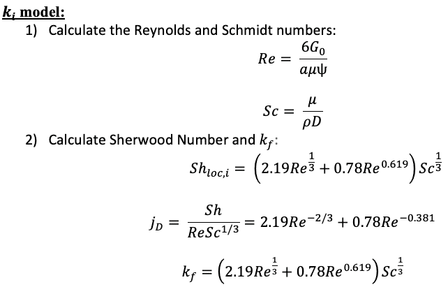
Screenshot 2022-05-19 at 15.06.20.png


So we calculate the Re and Sc numbers. Then the mass transfer coefficient ##k_i## seems to be a function of just these two numbers, so why the need to calculate the Sherwood number? And is Sh actually equal to ##k_f##?
 
Last edited:
Engineering news on Phys.org
  • #142
So I worked back through the mass transfer coefficient correlation derivation (my post above was a load of nonsense in hindsight, apologies). I almost have it but have uncertainty about which Sh number correlation to use. Heres the derivation (I just read back over the heat transfer coefficient derivation you did as its analogous to the mass transfer coefficient):

1) Define Sc and Re
##Re = \frac{6G_0}{a\mu\Psi}##
##Sc = \frac{\mu}{\rho D}##

2) Define the sherwood number
##Sh = \frac{k_id_p}{\rho_mD_{ab}}##

I took this one from BSL. I know you defined another Sh number earlier which was:
##Sh_{loc,i}=\frac{k_iD_p}{(1-\epsilon_g)D_i\psi}##

Its easy to interchange between the two but I am not sure of the reason to use one over the other

Anyway

3) Defining the CC factor ##j_D## as:
##j_D = ShRe^{-1}Sc^{-1/3}##

4) And the same specifically for packed beds:
##j_D = 2.19Re^{-2/3} + 0.78Re^{-0.381}##

5) Letting 3 equal to 4 and solving for k_i:
##k_i = (2.19Re^{1/3} + 0.78Re^{0.619})Sc^{1/3}D_{a,b}\frac{\rho}{d_p}##

Is this correct? I can easily sub in your Sh number instead of the BSL one, but what is the reason you did not use the BSL one?
 
  • #143
casualguitar said:
So I worked back through the mass transfer coefficient correlation derivation (my post above was a load of nonsense in hindsight, apologies). I almost have it but have uncertainty about which Sh number correlation to use. Heres the derivation (I just read back over the heat transfer coefficient derivation you did as its analogous to the mass transfer coefficient):

1) Define Sc and Re
##Re = \frac{6G_0}{a\mu\Psi}##
##Sc = \frac{\mu}{\rho D}##

2) Define the sherwood number
##Sh = \frac{k_id_p}{\rho_mD_{ab}}##

I took this one from BSL. I know you defined another Sh number earlier which was:
##Sh_{loc,i}=\frac{k_iD_p}{(1-\epsilon_g)D_i\psi}##

Its easy to interchange between the two but I am not sure of the reason to use one over the other

Anyway

3) Defining the CC factor ##j_D## as:
##j_D = ShRe^{-1}Sc^{-1/3}##

4) And the same specifically for packed beds:
##j_D = 2.19Re^{-2/3} + 0.78Re^{-0.381}##

5) Letting 3 equal to 4 and solving for k_i:
##k_i = (2.19Re^{1/3} + 0.78Re^{0.619})Sc^{1/3}D_{a,b}\frac{\rho}{d_p}##

Is this correct? I can easily sub in your Sh number instead of the BSL one, but what is the reason you did not use the BSL one?
The approach I'm recommending is based on Reynolds analogy, and I think it is better. I don't think that BSL considered this.

I believe your eon 5 is correct if dp is calculated by the definition in BSL.
 
  • #144
Chestermiller said:
The approach I'm recommending is based on Reynolds analogy, and I think it is better. I don't think that BSL considered this.

I believe your eon 5 is correct if dp is calculated by the definition in BSL.
Hmm I'm taking the characteristic length from the Sherwood number ##l_0## to be ##d_p##, the particle diameter. Why would dp be calculated using the BSL definition? Or have I misunderstood. The units for ##k_i## I have are ##mol/m2.s## not ##m/s## so I guess I am mistaken somewhere here

Also I'm effectively finished the function write ups and plots. I have the mass transfer coefficient one to confirm correct, then the mass deposition one is built on this so I have that also. Besides that I have two small questions regarding ##U_b## and ##U_g##

So ##U_b## will be a constant times the thermal conductivity divided by the particle diameter. This constant is ##\beta## I presume, which is equal to 10 for spheres, meaning that we would get ##U_b = \frac{\beta k_p}{d_p}##?

For ##U_g## we can evaluate this at the bulk gas temperature. I have taken the exact same correlation as we had in the previous model. However you mentioned we would have a correction factor involving viscosity at the interface this time? Why would we have this?
 
  • #145
casualguitar said:
Hmm I'm taking the characteristic length from the Sherwood number ##l_0## to be ##d_p##, the particle diameter. Why would dp be calculated using the BSL definition? Or have I misunderstood. The units for ##k_i## I have are ##mol/m2.s## not ##m/s## so I guess I am mistaken somewhere here
I had this worked out a few weeks ago, but don't quite remember now. You need to look at the table in BSL that has various versions of this in there. If I remember correctly, it is almost certainly the ##mol/m2.s## that we should be using. You need to play with the different versions until you arrive at the one that makes sense to you.
casualguitar said:
Also I'm effectively finished the function write ups and plots. I have the mass transfer coefficient one to confirm correct, then the mass deposition one is built on this so I have that also. Besides that I have two small questions regarding ##U_b## and ##U_g##

So ##U_b## will be a constant times the thermal conductivity divided by the particle diameter. This constant is ##\beta## I presume, which is equal to 10 for spheres, meaning that we would get ##U_b = \frac{\beta k_p}{d_p}##?
Yes, I think so.
casualguitar said:
For ##U_g## we can evaluate this at the bulk gas temperature. I have taken the exact same correlation as we had in the previous model. However you mentioned we would have a correction factor involving viscosity at the interface this time? Why would we have this?
See BSL section on heat transfer for turbulent flow in a pipe.
 
  • #146
Chestermiller said:
The approach I'm recommending is based on Reynolds analogy, and I think it is better. I don't think that BSL considered this.

I believe your eon 5 is correct if dp is calculated by the definition in BSL.
Ok got it I think. So using BSLs Sherwood number is ok, however the Reynolds analogy approach you used is better, meaning that ##k_i## would go from this with the BSL Sherwood number of ##Sh_{loc,i} = \frac{k_id_p}{\rho_mD_{ab}}##:
$$k_i = (2.19Re^{1/3} + 0.78Re^{0.619})Sc^{1/3}D_{a,b}\frac{\rho}{d_p}$$

To this, with your Sherwood number of ##Sh_{loc,i}=\frac{k_id_p}{(1-\epsilon_g)D_i\psi}##:
$$k_i = (2.19Re^{1/3} + 0.78Re^{0.619})Sc^{1/3}(1-\epsilon_g)D_i\frac{\psi}{d_p}$$

How would I assess which Sh correlation is better? I could plot one against the other for a range of ##k_i## values and see if they are almost equivalent. However if one returns appreciably higher values than the other I am not sure how to assess which is the better of the two
 
  • #147
Chestermiller said:
You need to play with the different versions until you arrive at the one that makes sense to you.
Yes any version I have tried has produced ##mol/m^2.s## so I'll go with this for now unless I see an inconsistency
Chestermiller said:
Yes, I think so.
Chestermiller said:
See BSL section on heat transfer for turbulent flow in a pipe.
Great, will do that this morning

Edit: Found those correlations. They give the laminar (Re<2100) and highly turbulent flow equations (Re>20000). The transition flow region is only available from a graph (no equation provided I don't think). The Re number for this system seems to be in the region of 20000 or so anyway, so for simplicity I will take the turbulent flow equation rather than extracting the relevant equation from the graph. That equation for forced convection and turbulent flow in tubes (and L/D > 10) is:
$$Nu_{ln} = 0.026Re^{0.8}Pr^{1/3}\frac{\mu_b}{\mu_0}^{0.14}$$
where ##\mu_b## is the bulk viscosity and ##\mu_0## is the surface viscosity which are I guess evaluated at the solid and fluid temperatures respectively?

So, this would mean the new ##U_g## heat transfer coefficient would be:
$$U_g = 0.026Re^{0.8}Pr^{1/3}\frac{\mu_b}{\mu_0}^{0.14}\frac{k_g}{d_p}$$

For reference, the previous model HTC was:
$$U_g = (2.19Re^{1/3} + 0.78Re^{0.66})Pr^{1/3}\frac{k_g}{d_p}$$
 
Last edited:
  • #148
Lastly, regarding the units of ki, any equation with ki in it shows that the unit of ki is ##mol/m^2.s##. However, the molar desublimation rate formula ##\dot{M}_i^"=k_i\left(\frac{Py_i-p_i(T_I)}{RT_I}\right)\tag{1}## suggests that the units are ##m/s##. If this is correct, is there an equivalent molar desublimation rate equation that would use units of mol/m2.s for ki?

For reference, my units are:
##k_i## = ##mol/m^2.s##
##P## = ##Pa##
##y_i## = ##mol/mol##
##R## = ##J/mol.K##
##T## = ##K##
 
  • #149
casualguitar said:
Yes any version I have tried has produced ##mol/m^2.s## so I'll go with this for now unless I see an inconsistencyGreat, will do that this morning

Edit: Found those correlations. They give the laminar (Re<2100) and highly turbulent flow equations (Re>20000). The transition flow region is only available from a graph (no equation provided I don't think). The Re number for this system seems to be in the region of 20000 or so anyway, so for simplicity I will take the turbulent flow equation rather than extracting the relevant equation from the graph. That equation for forced convection and turbulent flow in tubes (and L/D > 10) is:
$$Nu_{ln} = 0.026Re^{0.8}Pr^{1/3}\frac{\mu_b}{\mu_0}^{0.14}$$
where ##\mu_b## is the bulk viscosity and ##\mu_0## is the surface viscosity which are I guess evaluated at the solid and fluid temperatures respectively?

So, this would mean the new ##U_g## heat transfer coefficient would be:
$$U_g = 0.026Re^{0.8}Pr^{1/3}\frac{\mu_b}{\mu_0}^{0.14}\frac{k_g}{d_p}$$

For reference, the previous model HTC was:
$$U_g = (2.19Re^{1/3} + 0.78Re^{0.66})Pr^{1/3}\frac{k_g}{d_p}$$
No. No. The correlation you chose is for flow in a pipe, not a packed bed. You should continue to use the packed bed correlation, but just apply the wall viscosity correction.
 
  • #150
Chestermiller said:
No. No. The correlation you chose is for flow in a pipe, not a packed bed. You should continue to use the packed bed correlation, but just apply the wall viscosity correction.
Ah ok so it would be ##U_{g,NEW} = U_{g,OLD}*\frac{\mu_b}{\mu_0}^{0.14}##?
 
  • #151
Hi Chet, just to be clear on the ##k_i## units question, what I mean is that all of the correlations say that the units of ##k_i## are ##mol/m^2.s##, but, the desublimation rate equation says the units of ##k_i## are ##m/s##.

Equations that say ##k_i## unit is mol/m2.s:
##Sh_{loc,i} = \frac{k_id_p}{\rho_mD_{ab}}##
##Sh_{loc,i}=\frac{k_id_p}{(1-\epsilon_g)D_i\psi}##

Equation that says ##k_i## unit is m/s:
##\dot{M}_i^"=k_i\left(\frac{Py_i-p_i(T_I)}{RT_I}\right)##
 

Attachments

  • Screenshot 2022-05-23 at 16.15.39.png
    Screenshot 2022-05-23 at 16.15.39.png
    2 KB · Views: 47
  • #152
Hi Chet, by any chance would you have a source for the molar deposition rate equation (its possibly a variation of the Hertz-Knudsen equation)? I want to look into why the units don't seem to match up for ki in the Sherwood number correlations and ki in the molar deposition rate equation

Edit: any variation of this equation I have found has had a square root and pi in it which seems quite different to what we're using currently M˙i"=kiPyi−pi(TI)RTI

Edit: The closest equation I could find to our one is this:
Screenshot 2022-05-24 at 09.43.20.png

v is in kg/s rather than mol/m2.s here, I haven't managed to find the equation you used just yet (still looking)
 
Last edited:
  • #153
My apologies for the multiple posts. Is it possible that this equation ##\dot{M}_i^"=k_i\left(\frac{Py_i-p_i(T_I)}{RT_I}\right)## is missing a molar volume term on the right hand side (units of m3/mol). If so, then it essentially becomes ##\dot{M}_i^"=k_i\left(\frac{Py_i-p_i(T_I)}{RT_I}\right)*\rho_m## which is ##k_i*\frac{PV}{nRT}##. The brackets are dimensionless and this would mean that ##k_i## would have the same units as ##M_i''##, and this would line up with the units of ##k_i## in the sherwood number correlations
 
Last edited:
  • #154
casualguitar said:
Lastly, regarding the units of ki, any equation with ki in it shows that the unit of ki is ##mol/m^2.s##. However, the molar desublimation rate formula ##\dot{M}_i^"=k_i\left(\frac{Py_i-p_i(T_I)}{RT_I}\right)\tag{1}## suggests that the units are ##m/s##. If this is correct, is there an equivalent molar desublimation rate equation that would use units of mol/m2.s for ki?

For reference, my units are:
##k_i## = ##mol/m^2.s##
##P## = ##Pa##
##y_i## = ##mol/mol##
##R## = ##J/mol.K##
##T## = ##K##
If we write the equation ##\dot{M}_i^"=k_i\left(\frac{Py_i-p_i(T_I)}{RT_I}\right)\tag{1}## as $$\dot{M}_i^"=k_ic_I(y_i-p_i(T_I)/P)$$where ##c=\frac{P}{RT_I}##, then we can write $$\dot{M}_i^"=K_i(y_i-p_i(T_I)/P)$$

By analogy to Eqn. 14.5-6 of BSL, $$Sh=\frac{K_iD_p}{cD_i(1-\epsilon)\psi}$$Combining these gives $$\dot{M}_i^"=Sh \frac{c_ID_i(1-\epsilon)\psi}{D_p}(y_i-p_i(T_I)/P)$$
 
  • #155
Chestermiller said:
If we write the equation ##\dot{M}_i^"=k_i\left(\frac{Py_i-p_i(T_I)}{RT_I}\right)\tag{1}## as $$\dot{M}_i^"=k_ic_I(y_i-p_i(T_I)/P)$$where ##c=\frac{P}{RT_I}##, then we can write $$\dot{M}_i^"=K_i(y_i-p_i(T_I)/P)$$

By analogy to Eqn. 14.5-6 of BSL, $$Sh=\frac{K_iD_p}{cD_i(1-\epsilon)\psi}$$Combining these gives $$\dot{M}_i^"=Sh \frac{c_ID_i(1-\epsilon)\psi}{D_p}(y_i-p_i(T_I)/P)$$
Thats interesting. What you did above shows that ##M_i''## has the same units as ##K_i##. Issue solved then. Great! It looks like you did the same thing I did (there was a density factor I had not considered). I have this written up in code form so we're almost there on the functions front also. I have pretty much everything plotted for ranges of dependent variables also

Regarding the gas interface heat transfer coefficient ##U_g##, you mentioned I should continue to use the Nu correlation for flow in a packed bed, and add the wall viscosity correction. By this, do you mean:
##U_{g,NEW} = U_{g,OLD}*\frac{\mu_b}{\mu_0}^{0.14}##

Besides that question I think that's all issues solved for now. I just need to code up the last few heat transfer related functions (QgI, QIb, etc)
 
Last edited:
  • #156
casualguitar said:
Thats interesting. What you did above shows that ##M_i''## has the same units as ##K_i##. Issue solved then. Great! It looks like you did the same thing I did (there was a density factor I had not considered). I have this written up in code form so we're almost there on the functions front also. I have pretty much everything plotted for ranges of dependent variables also

Regarding the gas interface heat transfer coefficient ##U_g##, you mentioned I should continue to use the Nu correlation for flow in a packed bed, and add the wall viscosity correction. By this, do you mean:
##U_{g,NEW} = U_{g,OLD}*\frac{\mu_b}{\mu_0}^{0.14}##

Besides that question I think that's all issues solved for now. I just need to code up the last few heat transfer related functions (QgI, QIb, etc)
It's only an approximate thing. The viscosity term is only going to be a minor correction.
 
  • #157
Chestermiller said:
It's only an approximate thing. The viscosity term is only going to be a minor correction.
Perfect. Sure. This correction is in there now anyway. I'm tempted to post plots of all the main functions (Re, Sc, Pr, ki, U_g, etc) for suitable ranges of dependent variables later today to be sure they're ok before moving on

Actually one thing I noticed in writing the code for these functions is that there are 'layers' of functions. For example, viscosity is dependent on temperature, Reynolds number is dependent on viscosity, the mole transfer coefficient is dependent on the Reynolds number, and the molar deposition rate is dependent on the mole transfer coefficient.

This makes defining functions a bit messy in that I have for example the molar deposition rate function as a function of T, the sherwood number, the mass transfer coefficient, the mole fraction and the diffusion coefficient. I am tempted to look for a set of 'basis' variables that all functions are dependent on. For example, if I have every function as a function of temperature and the molar flow, would this be enough to calculate everything in any 'layer'? (assuming constants like P and ##y_i## are defined elsewhere). For now I will finish off these plots but it looks like finding this common basis would be useful for code simplicity
 
  • #158
Hi Chet, issue above resolved after chatting with a postdoc. Looks like the standard/OOP approach is to not do what I was thinking of doing above. This is fine as my code is already in this format anyway

One question - did we agree that ##Ug = h_{fs}##? I know in the last model we had the lumped parameter approach where we had ##\frac{1}{h} = \frac{1}{h_{fs}} + \frac{dp}{k*beta}## however here we are saying ##h = h_{fs}##?

Every function is written up now, and most plots are done. I've been able to check any of the thermodynamic property functions via literature data, however there are some other plots I'd like to check with you if possible. Also, most parameters have a number of dependent variables, so I would like to ask you which dependent variable is most insightful to vary for the plots. Here are my thoughts on possible plots and dependent variables I would vary within a range to create the plots. In the format '(The function output -> the variable being varied)':

Reynolds number -> molar flow
Prandtl number -> viscosity
Sherwood number -> mass transfer coefficient
Nusselt number -> ##h_{fs}##
Schmidt number -> viscosity
Mass transfer coefficient -> Reynolds number
Molar deposition rate -> mass transfer coefficient
##h_{fs}## -> Reynolds number

Working on these plots this morning. If you think there are other useful plots at this stage, or that there are better dependent variables to vary than the ones I chose just let me know
 
  • #159
casualguitar said:
Hi Chet, issue above resolved after chatting with a postdoc. Looks like the standard/OOP approach is to not do what I was thinking of doing above. This is fine as my code is already in this format anyway

One question - did we agree that ##Ug = h_{fs}##? I know in the last model we had the lumped parameter approach where we had ##\frac{1}{h} = \frac{1}{h_{fs}} + \frac{dp}{k*beta}## however here we are saying ##h = h_{fs}##?
##h_{fs}## is the heat transfer coefficient on the gas side, right?
Also, I think in this model we are calling the heat transfer coefficient on the gas side, the heat transfer coefficient on the solid bed side, and the overall heat transfer coefficient as ##U_g##, ##U_b##, and U. I'm not really sure. I lost track of the nomenclature we are using. You need to go back to my posts.
casualguitar said:
Every function is written up now, and most plots are done. I've been able to check any of the thermodynamic property functions via literature data, however there are some other plots I'd like to check with you if possible. Also, most parameters have a number of dependent variables, so I would like to ask you which dependent variable is most insightful to vary for the plots. Here are my thoughts on possible plots and dependent variables I would vary within a range to create the plots. In the format '(The function output -> the variable being varied)':

Reynolds number -> molar flow
Prandtl number -> viscosity
Sherwood number -> mass transfer coefficient
Nusselt number -> ##h_{fs}##
Schmidt number -> viscosity
Mass transfer coefficient -> Reynolds number
Molar deposition rate -> mass transfer coefficient
##h_{fs}## -> Reynolds number

Working on these plots this morning. If you think there are other useful plots at this stage, or that there are better dependent variables to vary than the ones I chose just let me know
The comparisons that make sense to me are in terms of the dimensionless groups, say ##Nu/Pr^{1/3}## vs Re (say comparing the correlation for turbulent flow in a tube to that in a packed bed).
 
  • #160
Chestermiller said:
Also, I think in this model we are calling the heat transfer coefficient on the gas side, the heat transfer coefficient on the solid bed side, and the overall heat transfer coefficient as Ug, Ub, and U. I'm not really sure. I lost track of the nomenclature we are using. You need to go back to my posts.
Yep looking back at those posts we are doing this
Chestermiller said:
The comparisons that make sense to me are in terms of the dimensionless groups, say Nu/Pr1/3 vs Re (say comparing the correlation for turbulent flow in a tube to that in a packed bed).
Almost finished with those other plots, so I'll add this one in then also. What information does a Nu/Pr^1/3 vs Re plot actually tell us? I suppose it can tell you how dominant convective heat transfer is for a range of Re values?

Edit: Will add all of these plots first thing tomorrow. If there are any other useful ones I can easily plot these two as I have functions for everything we would need to calculate now
 
  • #161
Just posting some plots here:

Molar flow vs Reynolds number (using system specific dimensions):
Screenshot 2022-05-26 at 12.17.44.png

Reynolds Number vs Mass Transfer Coefficient for CO2 and H2O:
Screenshot 2022-05-26 at 12.18.13.png


Reynolds Number vs Nu/Pr^1/3:
Screenshot 2022-05-26 at 12.18.35.png


If these look ok to you I think it's about time to start adding these functions into the simulation? Would you recommend any general order for adding these functions in? i.e. should I leave out any functions (and leave some constants) for now, or just go straight for adding them all in?
 
  • #162
casualguitar said:
Just posting some plots here:

Molar flow vs Reynolds number (using system specific dimensions):
View attachment 301954
Reynolds Number vs Mass Transfer Coefficient for CO2 and H2O:
View attachment 301955

Reynolds Number vs Nu/Pr^1/3:
View attachment 301956

If these look ok to you I think it's about time to start adding these functions into the simulation? Would you recommend any general order for adding these functions in? i.e. should I leave out any functions (and leave some constants) for now, or just go straight for adding them all in?
What is your judgment on this? My rule of thumb for modeling is always "start simple and build in complexity."
 
  • #163
Chestermiller said:
What is your judgment on this? My rule of thumb for modeling is always "start simple and build in complexity."
I do agree with this, and in addition it would be nice to start with a simple model that we can 'validate' against another model or against what we would intuitively expect to happen.

If we were to look at the mole fraction of co2/h2o in a single tank versus time, what trend would we expect?

I guess given that the ambient stream is hitting a cold bed we would see a yCO2 and yH2O spikes, and then when this bed heats up again the mole fractions would gradually decrease to zero?

If this is true, it at least offers some form of sanity checking.

As for simplifying it down initially though, we would need to implement the minimum amount of functions that allows for this trend to be seen.

It seems that the molar deposition rate is essential here (can't have this as a constant). Other possible requirements are ##Q_{IB}## and ##Q_{GI}##

What about leaving everything (all property functions and heat related functions) as constants, and just implementing variable ##M_i''## for a single tank?

Edit: Also in addition why the interest in a Nu/Pr^1/3 plot? What information does this convey?

Edit: Lastly just posting the actual equations here to bring them forward:
Screenshot 2022-05-26 at 16.10.24.png
 
Last edited:
  • #164
casualguitar said:
I do agree with this, and in addition it would be nice to start with a simple model that we can 'validate' against another model or against what we would intuitively expect to happen.

If we were to look at the mole fraction of co2/h2o in a single tank versus time, what trend would we expect?

I guess given that the ambient stream is hitting a cold bed we would see a yCO2 and yH2O spikes, and then when this bed heats up again the mole fractions would gradually decrease to zero?

If this is true, it at least offers some form of sanity checking.

As for simplifying it down initially though, we would need to implement the minimum amount of functions that allows for this trend to be seen.

It seems that the molar deposition rate is essential here (can't have this as a constant). Other possible requirements are ##Q_{IB}## and ##Q_{GI}##
No, but you can impose constant heat transfer- and mass transfer coefficients.
casualguitar said:
What about leaving everything (all property functions and heat related functions) as constants, and just implementing variable ##M_i''## for a single tank?
Try it and see how it plays out.
casualguitar said:
Edit: Also in addition why the interest in a Nu/Pr^1/3 plot? What information does this convey?
It would be interesting to compare this with the relationship with the corresponding variation for turbulent flow in a pipe.
casualguitar said:
Edit: Lastly just posting the actual equations here to bring them forward:
View attachment 301961
I think these are OK. Recheck the algebra to be sure.
 
  • #165
Chestermiller said:
No, but you can impose constant heat transfer- and mass transfer coefficients.
Ah nice, yes that sounds good. It means that temperature, heat transfer rate an molar deposition rate are all that will vary in this basic model. I guess this will be enough to see the yCO2 and yH2O trends
Chestermiller said:
Try it and see how it plays out.
Will do this that morning then
Chestermiller said:
It would be interesting to compare this with the relationship with the corresponding variation for turbulent flow in a pipe.
Can do. Why would this be interesting? It would quantify the effect of the packing on heat transfer coefficient I suppose
 
  • #166
casualguitar said:
Ah nice, yes that sounds good. It means that temperature, heat transfer rate an molar deposition rate are all that will vary in this basic model. I guess this will be enough to see the yCO2 and yH2O trends

Will do this that morning then

Can do. Why would this be interesting? It would quantify the effect of the packing on heat transfer coefficient I suppose
Hi Chet, have all functions etc for the current 'constant heat and mass transfer coefficient' model in the model. The model is giving some errors etc so I'm currently debugging these. Will post a condensed version of the initial conditions and output if I can't debug it
 
  • #167
casualguitar said:
Hi Chet, have all functions etc for the current 'constant heat and mass transfer coefficient' model in the model. The model is giving some errors etc so I'm currently debugging these. Will post a condensed version of the initial conditions and output if I can't debug it
I haven't solved this yet, but I did find something odd. Solve_ivp offers a number of integrators (LSODA, Radau, RK45, RK23, DOP853, BDF). I tried a few and they all seem to return very different results. Actually all of them show the gas temperature reaching temperatures that are not present in the system at all which indicates I'm doing something wrong anyway, but regardless I didn't expect the output from each integrator do vary this much
 

Attachments

  • Screenshot 2022-05-31 at 08.50.36.png
    Screenshot 2022-05-31 at 08.50.36.png
    12.2 KB · Views: 44
  • #168
casualguitar said:
I haven't solved this yet, but I did find something odd. Solve_ivp offers a number of integrators (LSODA, Radau, RK45, RK23, DOP853, BDF). I tried a few and they all seem to return very different results. Actually all of them show the gas temperature reaching temperatures that are not present in the system at all which indicates I'm doing something wrong anyway, but regardless I didn't expect the output from each integrator do vary this much
For reference, these are the initial, boundary, and constant values I'm using. Anything stand out here to you as being a value that is outside its typical range?

n = 5 #number of tanks
rho0CO2 = 1.1 #initial density of CO2 in bed (mol/m3)
rho0H2O = 1.1 #initial density of h2o in bed (mol/m3)
y0CO2 = 0 #initial gas phase mole fraction of CO2 in bed (mol/mol)
y0H2O = 0 #initial gas phase mole fraction of h2o in bed (mol/mol)
M0CO2 = 0.0 #initial solid CO2 moles deposited on bed (mol/m2)
M0H2O = 0.0 #initial solid h2o moles deposited on bed (mol/m2)
Tg0 = 150 #initial gas temperature (K)
Tb0 = 150 #initial bed temperature (K)
A_C = 0.005 #cross sectional area (m2)
A_s = 267 #specific surface area of solid (m2/m3)
h_vap_h2o = 40650 (J/mol)
v_desublimation_co2 = 26000 (J/mol)
k_s = 18 #solid heat capacity (W/m.K)
dz = 0.01
U_b = 100 #bed heat transfer coefficient (W/m2.K)
U_g = 200 #gas phase heat transfer coefficient (W/m2.K)
cp_CO2 = 45 #co2 heat capacity (J/mol.K)
cp_H2O = 45 #h2o heat capacity (J/mol.K)
ki_co2 = 8 #co2 mass transfer coefficient (mol/m2.s)
ki_h2o = 16 #h2o Mass Transfer coefficient (mol/m2.s)
m_co2 = rho0CO2*dz*A_C (value of 5*10^-5)
m_h2o = rho0H2O*dz*A_C (value of 5*10^-5)
M_al = 72.2 (mol/tank) (about 7kg/tank)

#Boundary conditions
mol_in = 0.5 #mol/s
y_co2_in = 0.1 #mol/mol
y_h2o_in = 0.01 #mol/mol
T_in = 220 #K
 
  • #169
casualguitar said:
For reference, these are the initial, boundary, and constant values I'm using. Anything stand out here to you as being a value that is outside its typical range?

n = 5 #number of tanks

casualguitar said:
rho0CO2 = 1.1 #initial density of CO2 in bed (mol/m3)
rho0H2O = 1.1 #initial density of h2o in bed (mol/m3)
What are these supposed to represent? I thought there is no water or CO2 deposited on the bed initially, and there is no water or CO2 in the gas phase initially.
casualguitar said:
y0CO2 = 0 #initial gas phase mole fraction of CO2 in bed (mol/mol)
y0H2O = 0 #initial gas phase mole fraction of h2o in bed (mol/mol)
M0CO2 = 0.0 #initial solid CO2 moles deposited on bed (mol/m2)
M0H2O = 0.0 #initial solid h2o moles deposited on bed (mol/m2)
Tg0 = 150 #initial gas temperature (K)
Tb0 = 150 #initial bed temperature (K)
A_C = 0.005 #cross sectional area (m2)
Bed diameter = 8 cm?
casualguitar said:
A_s = 267 #specific surface area of solid (m2/m3)
Please provide the calculation which led to this.
casualguitar said:
h_vap_h2o = 40650 (J/mol)
v_desublimation_co2 = 26000 (J/mol)
k_s = 18 #solid heat capacity (W/m.K)
thermal conductivity, not heat capacity
casualguitar said:
dz = 0.01
Units are meters? So total bed length is 0.05 m = 5 cm?
casualguitar said:
U_b = 100 #bed heat transfer coefficient (W/m2.K)
U_g = 200 #gas phase heat transfer coefficient (W/m2.K)
cp_CO2 = 45 #co2 heat capacity (J/mol.K)
cp_H2O = 45 #h2o heat capacity (J/mol.K)
cp of N2?
casualguitar said:
ki_co2 = 8 #co2 mass transfer coefficient (mol/m2.s)
ki_h2o = 16 #h2o Mass Transfer coefficient (mol/m2.s)
casualguitar said:
m_co2 = rho0CO2*dz*A_C (value of 5*10^-5)
m_h2o = rho0H2O*dz*A_C (value of 5*10^-5)
what are these?
casualguitar said:
M_al = 72.2 (mol/tank) (about 7kg/tank)
what is this?
casualguitar said:
#Boundary conditions
mol_in = 0.5 #mol/s
y_co2_in = 0.1 #mol/mol
y_h2o_in = 0.01 #mol/mol
T_in = 220 #K
 
  • #170
Chestermiller said:
Bed diameter = 8 cm?
Yes
Chestermiller said:
thermal conductivity, not heat capacity
Typo
Chestermiller said:
Units are meters? So total bed length is 0.05 m = 5 cm?
No the bed length is 2m. I've changed dz to 0.4m
Chestermiller said:
cp of N2?
Yes I haven't included this yet I just put in an approximate constant average value of the cp of N2,CO2,H2O

So to the problematic ones:
Chestermiller said:
What are these supposed to represent? I thought there is no water or CO2 deposited on the bed initially, and there is no water or CO2 in the gas phase initially.
Yes there is no deposited co2/water initially, and there is no co2/h2o present in the gas phase initially. I have set the deposited values to zero, but we're dividing by the molar holdup of CO2 and the molar holdup of h2o in 4/6 ODEs so I don't think I can let the molar holdup equal to zero. Therefore I've let it equal to the density of the vapour*cross sectional area*dz. This is actually wrong though also. The mass holdup is density of vapour * tank volume. Is it correct to say I can't have a molar holdup of zero ever because of this division issue?

Chestermiller said:
Please provide the calculation which led to this.
I think I had (and possibly still do) have an error here also. I just changed the calculation in the last few minutes. I still get an error in the simulation but the results do look better.

Specific surface area:
##S_A = V_{particle}/V_{bed} = \frac{2*d_p^3}{3*d_b^2h}##
where ##d_p## is the particle diameter, ##d_b## is the bed diameter and ##h## is the length of the bed
Chestermiller said:
what is this?
##M_{al}## is the total moles of solid alumina per tank

EDIT: So just to confirm, since that specific area fix, the gas temperature in the bed trends towards the inlet temperature, the gas fractions of co2/h2o trend towards the inlet mole fractions now
 
  • #171
A positive update-
Finally getting normal output for every variable (except bed temperature weirdly but I'll fix that). The time scale is obviously too short to reflect reality but here's an example plot of time vs gas temperature for each position (n=3):
Screenshot 2022-05-31 at 15.01.44.png

Working on that gas temperature bug now (the bed temperature seems to stay at the initial temperature)
 
  • #172
casualguitar said:
Yes there is no deposited co2/water initially, and there is no co2/h2o present in the gas phase initially. I have set the deposited values to zero, but we're dividing by the molar holdup of CO2 and the molar holdup of h2o in 4/6 ODEs so I don't think I can let the molar holdup equal to zero. Therefore I've let it equal to the density of the vapour*cross sectional area*dz. This is actually wrong though also. The mass holdup is density of vapour * tank volume. Is it correct to say I can't have a molar holdup of zero ever because of this division issue?
I don't understand this at all. Where do you divide by the molar holdup in your equations? And why does this have to include water and co2?
casualguitar said:
I think I had (and possibly still do) have an error here also. I just changed the calculation in the last few minutes. I still get an error in the simulation but the results do look better.

Specific surface area:
##S_A = V_{particle}/V_{bed} = \frac{2*d_p^3}{3*d_b^2h}##
where ##d_p## is the particle diameter, ##d_b## is the bed diameter and ##h## is the length of the bed
I don't understand this at all. The amount of particle surface area per unit volume of bed is ##\frac{6}{d_p}(1-\epsilon)## (assuming spherical particles).
casualguitar said:
##M_{al}## is the total moles of solid alumina per tank

EDIT: So just to confirm, since that specific area fix, the gas temperature in the bed trends towards the inlet temperature, the gas fractions of co2/h2o trend towards the inlet mole fractions now
I don't understand what this is saying.
 
  • #173
Chestermiller said:
I don't understand this at all. Where do you divide by the molar holdup in your equations? And why does this have to include water and co2?
The first term in the gas phase mole and heat balances ##m_{m,j}## is the molar holdup which is initially zero. When I divide across by this term (I do this when I'm setting up the ODEs in the solver), I'm left with a molar holdup in the denominator which is zero initially, unless I specify otherwise. No?
Screenshot 2022-06-01 at 15.07.11.png


Chestermiller said:
I don't understand this at all. The amount of particle surface area per unit volume of bed is 6dp(1−ϵ) (assuming spherical particles).
Yes sorry this is right I just quickly derived it by hand and got it wrong. Yes I agree its ##\frac{6}{d_p}(1-\epsilon)##

Chestermiller said:
The gas temperature should be high at the inlet and low downstream.
Yep that's also right (completely missed that). Interesting. Weird. I'll check this out
 
  • #174
casualguitar said:
Yep that's also right (completely missed that). Interesting. Weird. I'll check this out
Actually no this is fine. It shows the temperature profile vs time for the three tanks. We'd expect them all to be at T0 at time=0, and the first tank will be the first to rise up to the inlet temperature, etc
Screenshot 2022-06-01 at 15.49.12.png

However even though the trend is fine, for this simulation my inlet gas temperature is actually 220 so It shouldn't be levelling out at about 174. Bug somewhere
 
  • #175
casualguitar said:
The first term in the gas phase mole and heat balances ##m_{m,j}## is the molar holdup which is initially zero. When I divide across by this term (I do this when I'm setting up the ODEs in the solver), I'm left with a molar holdup in the denominator which is zero initially, unless I specify otherwise. No?
View attachment 302244
No. $$m_{m,j}=\frac{P}{RT_j}A\Delta z \epsilon$$This is the total number of moles of gas contained in tank j.
 

Similar threads

  • Materials and Chemical Engineering
13
Replies
454
Views
18K
  • Feedback and Announcements
Replies
2
Views
1K
  • Mechanical Engineering
Replies
0
Views
500
  • Other Physics Topics
Replies
6
Views
1K
  • Mechanical Engineering
Replies
1
Views
1K
  • Astronomy and Astrophysics
Replies
25
Views
1K
  • Mechanical Engineering
Replies
1
Views
1K
  • Differential Equations
Replies
1
Views
1K
  • STEM Academic Advising
Replies
8
Views
1K
  • Beyond the Standard Models
2
Replies
39
Views
1K
Back
Top