- #211
casualguitar
- 503
- 26
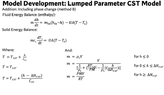
I don't. I can figure this out though. So to confirm, the two equations are the solid and energy balance here:Chestermiller said:Do you know how to solve this analytically (two linear coupled ODEs in two unknowns)?
Where ##h## and ##T_s## are the two unknowns, and where the ##h<=0## correlations will be used for ##T## and ##m##?