How Does the Hypersine Function Relate to the Expansion of the Universe?

  • Thread starter marcus
  • Start date
  • Tags
    Model
In summary, the hyperbolic sine is a function that splits the difference between the rising exponential function e^x and the exponential function run backwards, e^-x. It has a nice symmetry that the ordinary exponential function ex does not have. It has natural time scale which is opposite to the ordinary time scale. Distances, areas, and volumes grow according to powers of hypersine over time, and the scale factor a(t) tells us how big a distance is at some given time, compared with its present size. After a moment's inspection you can probably see the place around time 0.44 in our universe's history when distance growth stopped decelerating and gradually began to accelerate.
  • #36
Here is a picture for this entry in our (extremely abbreviated sketchy : ^) timeline.
0.44 switch from deceleration to acceleration [1.65]
I'm considering ways to say that which sound less technical. Up to a point the growth curve slope is decreasing down to about 45 degrees in the diagram, then the slope starts to increase. Could we say that this way?
0.44 growth stops easing and starts to steepen [1.65]

In the graph, the red curve keeps track of the upwards slope of the blue scale factor curve., which is very steep at the outset. The low-point on the swooping red curve corresponds to the minimum slope point of the blue. This is where deceleration ends and acceleration begins. It happens at time 0.44, when the height of the scale factor curve is about 0.6 (distances are about 60% of their present size)
I like using Lightcone7z to get graphs that illustrate moments in time, of the universe's expansion process. If anybody wants coaching on how to start using Lightcone7z to make graphs, just say, it's surprisingly easy.
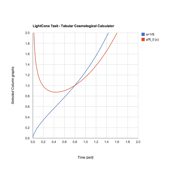
zeitswp.png

Let's try alternative wording for that short timeline. May sound dumb at first:
0.04 big star era over [8.6]View attachment 85356
0.234 most remote light arriving now[2.6] View attachment 85289
0.29 galaxy disk [2.2] View attachment 85383
0.44 growth starts to steepen [1.65] View attachment 85355
0.54 Earth [1.4]
0.59 microbial mat [1.3]
stroma2.jpg
stroma.jpg

0.66 "Great Oxygen Event" [1.2] View attachment 85360
0.77 "Cambrian explosion" [1.03] View attachment 85353
0.797 present [1]

Comparing these two:
0.234 today's light at farthest point on its way to us[2.6]
0.234 widest detour by light arriving here now[2.6]

comparing:
0.44 growth curve starts getting steeper [1.65]
0.44 growth stops easing and starts to steepen [1.65]
 
Last edited:
Space news on Phys.org
  • #37
Marcus, as always, a delight to read your explanations.

For some reason as I was reading your posts here, it dawned on me the the expansion outline [edges] of the diagram in Wikipedia here [Metric Expansion of Space]
https://en.wikipedia.org/wiki/Metric_expansion_of_space#Topology_of_expanding_space
is the one you are describing.
380px-CMB_Timeline300_no_WMAP.jpg


It hadn't occurerred to me before but the Wikipedia diagram apparently starts starts out with a representation of accelerated expansion early on and then glues on a[t]. Have I got that about right?
 
  • Like
Likes marcus
  • #38
I don't think the artist tried to make it to scale but it certainly is suggestive of the a(t) curve---as you said, glued on after the abrupt episode of inflation and having that characteristic inflection about halfway along---where convex (slowing) gives way to concave (speeding).
Nice illustration! I've seen a "bounce" version, looking a bit like an hour-glass. Don't have a link for it at the moment. I looked and found these (neither has the nice a(t) curve with inflection point).
bounfr.jpg


bounce.png
 
Last edited:
  • #39
I'm going to try illustrating this brief timeline with *thumbnails*of associated images. Time is given in zeits. The number in brackets is the wave stretch factor for light emitted at the given time, arriving now.
0.04 big star era over [8.6]
Reionz.jpg

0.234 some light that got here today lost ground until this point[2.6]
zeitpear.png

0.29 galaxy disk [2.2]
disk1.jpg

0.44 growth starts to steepen [1.65]
swoop.png

0.54 Earth [1.4]
0.59 microbial mat [1.3] View attachment 85478 View attachment 85479
0.66 "Great Oxygen Event" [1.2]
oxygen.jpg

0.766 "Cambrian explosion" [1.03]
cambr.jpg

.766 Rise of all major animal groups. Metazoan life abundant; trilobites dominant. First fish. No known terrestrial life. (Descriptions taken from the UC Berkeley Museum of Paleontology chart.

.768 First land plants, primitive fungi, sea weed appear. Diverse marine life: corals, molluscs, bivalves, echinoderms, etc.

.772 First spiders, scorpions, centipedes, early insects, vascular plants, jawed fish and large reefs appear.

.773 First amphibians. Extensive radiation of fish, land plants. Many corals, brachiopods and echinoderms.

.776 Echinoderms, bryozoans dominant in oceans. Early winged insects. First coal swamp forests.

.778 First reptiles, cockroaches and mayflies appear. Extensive coal swamp forests. Sponge reefs.

.780 Gymnosperms, amphibians dominant. Beetles, stoneflies appear. Major extinction of 95% of marine species and 50% of all animal families.

.783 Origin of mammals, dinosaurs and true flies. Less diverse marine fauna.

.785 Dinosaurs and gymnosperms dominate the land; feathered dinosaurs and birds appear. Radiation of marine reptiles.

.789 Marsupials, ants, bees, butterflies, flowering plants appear. Mass extinction of most large animals and many plants.

.793 Early placental mammals appear; first primates; modern birds.

.794 Early mammals abundant. Rodents, primitive whales and grasses appear.

.7948 Worldwide tropical rainforests. Pigs, cats, and rhinos appear. Dominence of snails and bivalves in the oceans.

.7957 Coevolution of insects and flowering plants. Dogs and bears appear.

.7967 Extensive radiation of flowering plants and mammals. First hominids appear.

0.797 NOWhttp://www.ucmp.berkeley.edu/education/explorations/tours/geotime/guide/geologictimescale.html
with dates in zeits added.
Start of Cambrian which I earlier wrote as 0.77, made more precise here as 0.766 zeit.

https://en.wikipedia.org/?title=Reionization
https://en.wikipedia.org/wiki/Microbial_mat .797 - 3.5/17.3
https://en.wikipedia.org/wiki/Cyanobacteria
https://en.wikipedia.org/wiki/Great_Oxygenation_Event .797 - 2.3/17.3
https://en.wikipedia.org/wiki/Cambrian_explosion
https://en.wikipedia.org/wiki/Opabinia
http://www.nature.com/articles/nature13068.epdf?referrer_access_token=7deHVh_Wh220hQSvedJIitRgN0jAjWel9jnR3ZoTv0NhbzmErbf5JCFwVjms9AMgLfLdw2FHTyrtNmaEuljV-DpsFhzftIBY7OMLYngSZP8MtbOlbXf7TGczR1bvmsm9G5FBIuErjZ4m2yDAew7QOCLCQbyLonsmDaNdu7QqCBechIAx7tcy7uRl9dKZ8KKgKYdZj76xiw9DzG_kLGaCpg==&tracking_referrer=www.nature.com
 
Last edited:
  • #40
To review the basic idea here, the aim is to visualize the standard cosmic model with the help of three automatic formulas---shown in a form that can be pasted into google which will then compute them. One of our formulas is for the "Hubble radius" R, so I had better define that. R is the size of distances which are growing at speed c. It gives a handle on the expansion rate. The larger R is---the farther out you have to look to see distances growing at speed c. The speed any distance is growing is proportional to its size---so its expansion speed in terms of c is simply its size divided by R.

Another of our formulas involves the size ratio S. We can designate times by how the sizes of distances and wavelengths then compared with their sizes now. Any given time is characterized by this size ratio.

Now/then size ratio (substitute any two different times for "now" and "then")
sinh(1.5*now)^(2/3)/sinh(1.5*then)^(2/3)

If we set "now" to be the present 0.797 ≈ 0.8 this ratio compares distances and wavelength sizes at present with their sizes at some other time t.
The numerator in this case is sinh(1.5*0.797) = 1.3115 ≈ 1.3
Let's denote by S(t) the size now compared with at time t. e.g. S = 2 means now twice as big as at time t. In Lightcone calculator S is termed the stretch factor.
S can be used to designate a time---e.g. the time t for which S(t) = 2 would be the time when wavelengths and distances were half their present size. So that coming from that time up to the present, distances and wavelengths would double.

The next formula is for the "Hubble radius" R(s) corresponding to a given value of S. Recall that R is the size of distances which are growing at speed c. The self-computing formula for R(s) is
((s/1.3)^3 + 1)^(-1/2)
This can be used to find the distance covered by light arriving with stretch S, in other words the present distance D(S) of the light from its source.
$$D(S) = \int_1^S R(s)ds = \int_1^S \frac{ds}{\sqrt{(s/1.3)^3 + 1}}$$

The third formula computes the time t in terms of the Hubble radius R at that time. Just replace R by a number between zero and one in this expression and paste into google. It will calculate the corresponding t(R).
ln((1+R)/(1-R)/3
$$t = \frac{1}{3} \ln\frac{1+R}{1-R}$$
 
Last edited:
  • #41
Trying the formulas out. Some exercises.
What's the wavelength and distance size ratio between:
the formation of our galaxy's disk and the formation of the Earth
the big star era and the start of acceleration
the appearance on Earth of the first microbes and the first reptiles

Time-marker events:
0.04 big star era over [S=8.6]
View attachment 85356
0.234 light that got here today lost ground until this point[S=2.6]
View attachment 85357
0.29 galaxy disk [2.2]
View attachment 85383
0.44 acceleration starts [1.65]
View attachment 85355
0.54 Earth forms [1.4]
0.59 microbes appear [1.3]
View attachment 85478
0.66 oxygen builds up [1.2]
View attachment 85360
0.766 Rise of all major animal groups [1.03]
View attachment 85353
.768 First land plants
.776 Early winged insects.
.778 First reptiles.
.783 Origin of mammals, dinosaurs.

Sample answer:
What's the size increase ratio between "Earth forms" and "First land plants"?
sinh(1.5*0.768)^(2/3)/sinh(1.5*0.54)^(2/3)
 
Last edited:
  • #42
More exercises to try out the formulas.

Some light comes in today from a galaxy which when it emitted the light was receding at speed c. So at first that light made zero progress.
How far from home is that light now?

Answer: the light is wavestretched by a factor of S=2.6. Put ((s/1.3)^3 + 1)^(-1/2) in for the integrand and set the limits at 1 and 2.6

Some light comes in today from some of the last "PopulationIII" stars, the big stars that formed before there were elements heavier than H and He.
How far is that light from home?
Answer: set the limits of integration at 1 and 8.6

Some light comes in today that started towards us at a time when our galactic disk was forming. How far from its source is that light?
Answer: set the limits of integration at 1 and 2.2

http://www.numberempire.com/definiteintegralcalculator.php
 
  • #43
Since we turned a page I'll bring forward the latest post with the three basic formulas in it. The aim is to visualize how the standard cosmic model works with the help of three formulas---in a form which will self-compute when pasted into google.

A definition: the "Hubble radius" R is the size of distances which are growing at speed c. It gives a handle on the slowness of expansion. The larger R is---the farther out you have to look to see distances growing at speed c. The speed any distance expands is proportional to its size---so its expansion speed in terms of c is simply its size divided by R.

We make considerable use here of this wavelength and distance size ratio
(substitute any two different times for "now" and "then")
sinh(1.5*now)^(2/3)/sinh(1.5*then)^(2/3)

A particular application involves setting "now" to be the present 0.797 ≈ 0.8. Then this ratio compares distances and wavelength sizes at present with their sizes at some earlier or later time t. The numerator in this case is sinh(1.5*0.797) = 1.3115 ≈ 1.3
Let's denote by S(t) the size now compared with at time t. e.g. S = 2 means now twice as big as at time t.

In Lightcone calculator S is termed the stretch factor. S can be used to designate a time---e.g. the time t for which S(t) = 2 would be the time when wavelengths and distances were half their present size. So that in coming from that time up to the present, distances and wavelengths would double.

The next formula is for the "Hubble radius" R(s) corresponding to a given value of S. Recall that R is the size of distances which are growing at speed c. The self-computing formula for R(s) is
((s/1.3)^3 + 1)^(-1/2)
This can be used to find the distance covered by light arriving with stretch S, in other words the present distance D(S) of the light from its source.
$$D(S) = \int_1^S R(s)ds = \int_1^S \frac{ds}{\sqrt{(s/1.3)^3 + 1}}$$

The third formula computes the time t when the Hubble radius R was some given value. Just replace R by a number between zero and one in this expression and paste into google. It will calculate the time corresponding to that Hubble radius.
ln((1+R)/(1-R)/3
$$t = \frac{1}{3} \ln\frac{1+R}{1-R}$$
 
  • #44
Geologists have identified 5 major mass extinctions (plus the current one caused by humans, which we do not discuss here, sometimes called the "sixth")
and all five occurred in the 700s. (on a millizeit scale, the present 0.797 is 797.)
They had various causes and they occurred in '71, '76, '82, '85, and '93.

The most severe of these five mass extinctions was the extinction of '82, which is called the Permian-Triassic (or P-Tr) extinction. It is almost unbelievable what a large percentage of then-existing species were wiped out.

The extinction of '93 (which eliminated non-bird dinosaurs) was quite mild by comparison. Geologists are changing the name of this one: it used to be called Cretaceous-Tertiary (abbreviated K-T) but now they want to call it Cretaceous-Paleogene abbreviated K-Pg.
https://en.wikipedia.org/wiki/Extinction_event

In chronological order the five major mass extinctions are:

Extinction of '71 Ordovician-Silurian (O-S)

Extinction of '76 Late Devonian (Late-D)

Extinction of '82 Permian-Triassic (P-Tr)

Extinction of '85 Triassic-Jurasic (Tr-J)

Extinction of '93 Cretaceous-Paleogene (K-Pg)
 
Last edited:
  • #45
Hypersine cosmic model has local PF roots going (as I recall) back to some posts by George Jones and Jorrie. George has a more formal-professional presentation here, called Redshift-Distance Relationships:

https://www.physicsforums.com/attachment.php?attachmentid=59214&d=1370171072

It's a 6 page PDF. The basic facts are well known: the sinh2/3(1.5t) function gives an excellent approximation to the real universe scale factor back in time to about t = 0.00001. So it's a practical model of expansion to calculate with over any timespan after the early universe when radiation was dominant over matter.

When cosmic-scale distances are all growing at speeds proportionate to their size the speed-to-size ratio a'(t)/a(t) at any given moment t is
cosh(1.5t)/sinh(1.5t).

That's the key thing and it is where some first-year calculus comes in. You have to take the derivative (slope) of sinh2/3(1.5t) and divide it by sinh2/3(1.5t). That gives the speed-to-size ratio, usually denoted H(t). It is what you have to multiply the size of a distance by to get the speed it's growing, at that moment. v(t) = H(t)D(t) Hubble's law of distance expansion.
 
Last edited:
  • #46
marcus said:
Hypersine cosmic model has local PF roots going (as I recall) back to some posts by George Jones and Jorrie. George has a more formal-professional presentation here, called Redshift-Distance Relationships:

https://www.physicsforums.com/attachment.php?attachmentid=59214&d=1370171072
That's a nice presentation, with equations in terms of time and graphs against redshift.

I have a small issue with George's section 6, Cosmological Horizon. It may be just semantics, but he calculates what we call the 'particle horizon' and his term might be confused with the 'cosmological event horizon' (or 'communication horizon', which is the largest proper distance that a signal emitted at time t can ever bridge), which is presently 16.5 Gly.

I may be wrong, but I also have a problem with:

George said:
(https://www.physicsforums.com/attachment.php?attachmentid=59214&d=1370171072, section 6)
The calculated value for dhorizon is somewhat larger than the accepted value of 46 billion
light-years because te should actually be the time from which we receive the Comic Microwave Background (CMB) radiation.

I think his value of 47.15 Gly (rather than the correct particle horizon distance of 46.3 Gly) stems from the approximation when ignoring radiation energy density in the pre-CMB era. The "CMB distance" is some 45.4 Gly.
 
  • #47
I noticed the same slight variation in terminology around "particle horizon" that you did. There's alway some variation in language, and it does risk causing confusion, but we both see what he's saying---having the integral written explicitly helps. Also, you're probably right about the different Gly values.

I'm happy this little project seems to be coming to fruition, and to tell the truth it is largely because of all the work you put into it (with your PF Insights piece but also including the zeit version of Lightcone, with its ability to plot curves!)

At present this thread is kind of insubstantial. I'm turning in for the night at this point but I'll see if I can think of directions it could go tomorrow. If you see some way to beef it up or give it more content, please have a go at it : ^)
 
Last edited:
  • #48
Jorrie, I was slow off the mark this morning you might not see this until tomorrow because of the timezone difference. An idea finally got settled in my head which I'd like to try. It follows up on what you said recently about concentrating where possible on the more observable measurable quantities.
What I noticed is that the scale factor a = 1/S = 1/(z+1) is just as observable as S and it's intuitively more like time. So suppose I do some Lightcone plots with a on the x-axis. Let me try using this graph to explain something:
deesforscale.png

Today there was a newcomer asking "how do we know the age of the universe?" a common question! And how do we know the particle horizon is 46 Gly? in words to that effect---radius of the observable region---farthest light can have traveled for the whole expansion age. Here is his thread:
https://www.physicsforums.com/threads/the-age-of-the-universe.827359/

Well that 46 Gly is the 2.67 that the blue curve hits. So how do you get the blue curve? The redshift-distance data (standard candles) falls along that curve. One could say so far mostly along the right half, e.g. from 0.4 to 1.0.

But we also have a nice data point on the left end too, that comes from the red curve. The temperature of the gas that emitted the CMB can be estimated on physical grounds, so can the actual size of pressure waves in the gas at the time CMB was emitted. Temperature tells us the scale factor back then, and comparing their present angular size in the sky with their real size then, tells their distance back then. That's the red curve. And dividing red curve height by scale factor a gives blue curve. It's admittedly complicated and involves assumptions, but there is a chain of inference based on observation that puts more data points on the blue curve.

Other observations come under the heading Baryon Acoustic Oscillation. I think I might leave the idea half developed at this point and go look at that newcomer's post where he asks (if you put it in zeit terms) how do we know the 2.67? and how do we know the 0.8? the latter being the expansion age.

I just checked back at your Part 4
https://www.physicsforums.com/insights/approximate-lcdm-expansion-simplified-math-part-4/
and see a bunch of graphs with scale factor a on the horizontal axis. That may have been what got me thinking along these lines. So much of the basic data supporting Cosmology falls along that blue curve---scalefactor-distance, which the Cosmologists plot backwards as the "redshift-distance" curve.

When light comes in it tells you what the scalefactor was when it was emitted.
So much of cosmology has to do with understanding how far the source of that light is from us now.
The blue curve. The model that is fitted to the scalefactor-distance data.
 
Last edited:
  • #49
We often get novice posts asking basic questions like "how do we know the present expansion age is 13.8 billion years?" and "how do we know the present observable range is 46 billion lightyears?" or words to that effect. Where do those numbers come from, on what observations are they based?
those are good questions.

Here's an example of someone asking those kinds of questions: https://www.physicsforums.com/threads/the-age-of-the-universe.827359/
"Can someone please explain this in details for me? Like how do we know the age of the universe?"

How would one try to answer that kind of basic question in the context of the hypersine version of the standard model?

Well given the present-day Hubble radius (which Hubble already in 1930s effectively measured) this is just a one parameter model. We simply adjust that parameter so as to get the best fit to the available data.
The data we're fitting is "redshift-distance" data, or more exactly "scalefactor-distance" data, which we can picture as data points consisting of two numbers (a, Dnow). The scale factor (i.e. size of distances compared with present) when the light was emitted and the light's present distance from its source.

The present-day Hubble radius is straightforward, almost trivial, to measure, based on comparatively nearby objects whose recession speed is indistinguishable from their redshift z. Wherever one can determine the distance to an object one simply divides D/z. Since z is a pure number this gives a distance--essentially the slope of a nearly straight line of data. That distance Rnow ≈ 14.4 Gly.

Taking that distance as given, there is only one adjustable parameter which I'll call tnow. It turns out that the best fit is achieved by setting tnow = 0.8, or to higher precision for some applications tnow = 0.797.

Let's say we choose the value 0.8, this amounts to choosing a TIME UNIT for the model and also longterm values for the Hubble time, expansion rate, and radius (all equivalent ways of talking about the same thing.)

Choosing tnow = 0.8 has the effect of setting our TIME UNIT = coth(1.5*0.8)*14.4 Gy ≈ 17.3 Gy
and our DISTANCE UNIT = coth(1.5*0.8)*14.4 GLy ≈ 17.3 GLy
It also has the side effect of establishing the expansion age as 0.8 time units, namely about 0.8*17.3 Gy.
All these things, and more, come from choosing a value of this one parameter.

Then we have to see how good the fit is to the data---the collection of scalefactor-distance data points.
That is where the Dnow curve comes in, that we showed earlier. Each slightly different choice of the parameter results in a slightly different curve. What was shown was the curve for 0.8.
 
Last edited:
  • #50
Imagine that a lot of distance-redshift data points are collected, or equivalently distance-scalefactor points and they are plotted on this graph to see how well the blue curve fits the data. This is how we decide what value to give the parameter tnow. Making it 0.8 gives the best fit.
So how exactly is that done? how do we try alternatives like 0.6, 0.7, 0.9, and 1.0?
deeferscale.png

Some light comes in and says its scalefactor at emission was some number "a" between 0 and 1. Now using each alternative tnow from 0.6 to 1.0 we calculate how far that light is now from its source. That's the curve. And also we can look at the observational data point (a, D) and see how well the curve matches up. So how is the curve generated, using the choice of tnow model parameter?

the D(a) value on the curve is calculated as an integral from a to one of a certain function (which depends on the parameter) and which tracks the step by step progress from the emission of the light to the present (a=1) and how much each step got expanded while the light was in transit.

I'll show the integrands for each parameter choice. They differ in height, so the areas under them differ in size. They predict different D distances for each given initial scalefactor "a" number. As it happens, the red curve--the one for parameter value 0.8 is the one with best fit. The others predict distances, for each given initial "a" which are either too big or too small:
SS13Aug.png

The formula for the integrand is a bit messy because we have to show how it depends on the parameter. Once you decide which parameter is right, say t = 0.8, you can simplify the formula considerably
 
Last edited:
  • #51
The integrands to give comparable distance answers need to have conversion factors to get all the outputs in the same unit. That is what the
0.83coth(1.5*0.6) out front is doing---it gets all the distances in lightzeits. In the case of t=0.8 the factor .83coth(1.5* .8) is just equal to one and has no effect. Here for example is the distance integral where the model parameter is chosen to be 0.6

[tex]D_{.6}(a) = .83\coth(1.5* .6)\int_a^1 x^{-2} (\sinh^{-2}(1.5* .6)x^{-3} + 1)^{-1/2} dx[/tex]

If we want to use numberempire.com or one of the other easy online integrators, then the function to be integrated would be pasted into the integrand box in this format:
.83*coth(1.5* .6)* x^(-2) (sinh(1.5* .6)^(-2)*x^(-3) +1)^(-1/2)
and then to calculate the other cases one would just change the .6 to .7, or to .9...

The limits of integration would of course be the numbers a and 1, for light that comes in today showing an initial scalefactor of a. IOW light that has been stretched by a factor of 1/a.
 
Last edited:
  • #52
My contention is that the accelerating rate of expansion of the universe is an illusion. I don't know how to put this into mathematical or geometric terms but it seems clear to me that if we have (say) three equidistant galaxies - the first being 1 distance from Earth, the second being double that 1 distance, and the third being triple that 1 distance, and we measure the redshift at time now, and give them 10 years to account for the expansion of the universe then measure the redshift again, it would appear that the more distant galaxy were accelerating away from Earth 3 times faster (or whatever) than the closest galaxy. However, if there were merely a constant rate of expansion between us and 1, and 1 and 2, and 2 and 3, we have to sum up the constant expansion rates. because we must add the constant rate of expansion between each to the constant rate of expansion between them. Thus we get the illusion of accelerating expansion the further a galaxy (or star) is away from us. However, if the rate of expansion is constant the sum of the constants gives us the same result as assuming that some unknown force is causing the acceleration, instead of the much more plausible explanation that the force that is causing the expansion is the same everywhere. The accelerating rate of expansion is simply an illusion caused by the failure to add the expansion between objects to the same rate of expansion between more distant objects due to the constant creation of space between objects..
 
  • #53
Hello JB, I think you are saying something very reasonable which I'll try to paraphrase as follows. The expansion RATE (properly understood as a speed-to-size ratio or a percentage growth rate) means that larger distances grow faster.

So the RATE could be constant, and if we focus on just one distance and keep track of it, its growth speed will increase over time simply because its SIZE increases over time.

The RATE could even be gradually declining, and if the decline was gradual enough we would still see the growth speed increase over time of that one distance we are tracking, because its size is increasing and the speed-to-size ratio, or percentage rate,. is nearly constant (even if slowly declining).

What we are describing is "near exponential growth" with a gradually declining growth rate.

So if I understand you, you are saying that if we think "acceleration" means increasing expansion rate then we are CONFUSED and under an ILLUSION. This is correct. You are not the only one who knows this. More or less any cosmologist or informed reader who follows the professional research literature knows this.

Actually the evidence suggests that the expansion rate has always been declining since very early times and according to standard model is expected to continue declining but more and more gradually so that it levels off at a positive rate.

At a certain point in the past (I don't recall what it is in billions of years but it was 0.36 times 17.3 billion years ago) the decline became gradual enough so that you would have seen acceleration on a distance by distance basis, as we discussed---the "near exponential growth" idea. For much of the time before that the decline in the rate was so drastic that you didn't even see the "illusory" acceleration---watching a single distance and seeing its speed change as it gets larger---its growth speed would actually decline over time even though it was getting larger because the rate was going down so drastically...

You might enjoy learning how to use Jorrie's calculator to plot curves
 
Last edited:
  • #54
growth.png

H is the expansion RATE which you can see has always been declining. In early times before time 0.4 very very steeply.
The blue curve (called the "scale factor" is the size of a generic distance normalized to equal 1 at the present. The present is 0.8.

You can see that the blue curve slope decreases until around time 0.44 and then it gradually begins to adopt a increasing slope "near exponetual growth" shape. In this plot, time 1.0 is year 17.3 billion. that turns out to be a convenient unit of time that makes the standard cosmic model equations exceptionally simple and easy to work with.
http://www.einsteins-theory-of-relativity-4engineers.com/LightCone7z/LightConeZ.html
To get curves you just go there and tick the button that says "chart" in the "Display as" options row, and press "calculate". You will get a chart like what I copied here but with 5 curves instead of two. There is a way to deselect the other 3 curves if you want to make it easier to read, but the main thing is to do the first thing of just getting the chart. Lightcone graphic cosmology calculator is user-friendly.
 
Last edited:
  • #55
The aim of this equivalent version of the standard LambdaCDM model is to have a ONE-STOP VERSION of standard cosmology (simplified by not worrying about the very early radiation-dominated era) and to have it as TRANSPARENT as possible.

You should be able to see how we arrive at the expansion age ("age of the universe" if you think there was no universe before start of expansion : ^).

That's what I mean by transparency: you should see how it is derived by fitting redshift-distance data measured using the various standard candles. Fairly directly. It should be easy.

You should be able to calculate the range of observation (the "particle horizon", the radius of the current observable region). You should be able to calculate for yourself that 46 billion ly. Or 2.7 lightzeit (in terms of our easy-to-use unit of time).
And see WHY that formula works: breaking down the light's trip into small steps each multiplied by how much the step gets expanded between then and now.

You should be able to calculate for yourself today's signal range---the "cosmic event horizon" the distance to the farthest galaxy we could reach by a signal sent today, with no limit on how long it takes to get there.
16.5 billion ly or in our terms 0.95 lightzeit. You may be able to see how the signal range is still increasing and gradually approaching a limit of exactly 1.0 natural distance unit.

It's the same integral, but with different limits: from present (sending) to infinity instead of from zero to the present(arrival).
 
Last edited:
  • #56
The model really has two parameters but the first one, Hnow, is a no-brainer. For nearby galaxies all the growth is effectively taking place at the present rate and a galaxy's redshift is a direct index of its distance growth speed as a fraction of c.
The second parameter is the non-trivial one obtained by fitting curve to data. The data can be redshift-luminosity, redshift-distance, scalefactor-distance. These are equivalent forms of the same information: luminosity is used to gauge distance, redshift z determines scale a = 1/(z+1) at time of emission. In this presentation we imagine the data to be (a, D) scalefactor-distance. and we want a curve D(a) that passes through those data points.

Here are some curves D.6(a) ...D1.0(a)
In each case the value of the curve at a is the integral from a to 1 of an integrand which depends on the parameter.
[tex]D_{.6}(a) = .83\coth(1.5* .6)\int_a^1 x^{-2} (\sinh^{-2}(1.5* .6)x^{-3} + 1)^{-1/2} dx[/tex]
[tex]D_{.7}(a) = .83\coth(1.5* .7)\int_a^1 x^{-2} (\sinh^{-2}(1.5* .7)x^{-3} + 1)^{-1/2} dx[/tex]
[tex]D_{.8}(a) = .83\coth(1.5* .8)\int_a^1 x^{-2} (\sinh^{-2}(1.5* .8)x^{-3} + 1)^{-1/2} dx[/tex]
[tex]D_{.9}(a) = .83\coth(1.5* .9)\int_a^1 x^{-2} (\sinh^{-2}(1.5* .9)x^{-3} + 1)^{-1/2} dx[/tex]
[tex]D_{1.0}(a) = .83\coth(1.5* 1.0)\int_a^1 x^{-2} (\sinh^{-2}(1.5* 1.0)x^{-3} + 1)^{-1/2} dx[/tex]
 
  • #57
I read today that the earliest known flowering plants were from 7 millizeits ago. the best fossil of one of them (Montsechia) was found just recently. It was a freshwater aquatic plant that thrived in what are now mountainous parts of Spain.
http://news.indiana.edu/releases/iu/2015/08/first-flower-angiosperms.shtml
https://www.iu.edu/~images/dams/479311_actual.jpg
Monts.jpg

Since the present, on our scale, is 797 millizeits, this puts the appearance of the first flowering plants at around 790 mz. this comes between the last two mass extinctions, that of 785 and that of 793 (which did for the non-bird dinosaurs.)
In a previous post I listed the 5 mass extinctions of the 700s.
marcus said:
Geologists have identified 5 major mass extinctions ...[which] occurred in the 700s. (on a millizeit scale, the present 0.797 is 797.)
They had various causes and they occurred in '71, '76, '82, '85, and '93.

The most severe of these five mass extinctions was the extinction of '82, which is called the Permian-Triassic (or P-Tr) extinction. It is almost unbelievable what a large percentage of then-existing species were wiped out.

The extinction of '93 (which eliminated non-bird dinosaurs) was quite mild by comparison. Geologists are changing the name of this one: it used to be called Cretaceous-Tertiary (abbreviated K-T) but now they want to call it Cretaceous-Paleogene abbreviated K-Pg.
https://en.wikipedia.org/wiki/Extinction_event

In chronological order the five major mass extinctions are:

Extinction of '71 Ordovician-Silurian (O-S)

Extinction of '76 Late Devonian (Late-D)

Extinction of '82 Permian-Triassic (P-Tr)

Extinction of '85 Triassic-Jurasic (Tr-J)

Extinction of '93 Cretaceous-Paleogene (K-Pg)
Montsechia vidalii was contemporanious with or earlier than the other earliest known angiosperm (flowering/seed producing plant) Archaefructus sinensis---an ancient freshwater plant that lived in China. Archefructus fossils are also dated around 790 mz.
 
Last edited:
  • #58
marcus said:
you can probably see the place around time 0.44 in our universe's history when distance growth stopped decelerating and gradually began to accelerate.
Hi marcus:

I calculated the value of a for q = 0, and came up with a = 0.606. The equation I used is derived as follows (I use the apostrophe for d/dt):
q =(def) a'' a / a'2 = - (H2 + H') / H2
q = 0 → H2 + H' = 0
H = H0 ( (1-Ωm) + Ωm a-3 ) 1/2
H2 = H02 (1-Ωm + Ωm a-3)
H' = H0 (1/2) (1-Ωm) + Ωm a-3 ) -1/2 (-3 Ωm) a-4 a'
H' = H0 (-3Ωm/2) ((1-Ωm) + Ωm a-3)-1/2 a-3 H = (-3Ωm/2) H02
H2 + H' = (1-Ωm) + Ωm a-3 - (3/2) Ωm a-3 = (1-Ωm) -(1/2) Ωm a-3
q = 0 → a = [(1/2) Ωm/(1-Ωm)]1/3
The value I used for Ωm = 0.308

Using the value 0.44 for t, I calculated a = ((1/2) (e3t/2 - e-3t/2))2/3 to get a = 0.631.

Did I misunderstand how to use the hypersine?
Did you use a different value for Ωm to calculate H?
Can you suggest another reason for the discrepancy?

Regards,
Buzz
 

Attachments

  • upload_2015-11-6_13-9-47.png
    upload_2015-11-6_13-9-47.png
    303 bytes · Views: 422
  • #59
thanks for the calculation! I have to go out to an appointment and can't give a proper response now, but I'll bet your calculation is right.
My figure of 0.44 could just be approximate and give a=.631 whereas your a = .606 could be more correct (given your assumptions about the inputs, which seem reasonable---don't have time to check right now).
Delighted to see you got into this thread, Buzz.
 
  • #60
Hi marcus:

I did a bit more calculating and came up with the value t = 0.304 to go with the value a = 0.606. Eyeballing the chart on post #2, the inflection point could be at t = 0.3

Regards,
Buzz
 
  • #61
Eyeballing a curve to find the inflection point can be hard esp if it is nearly linear for a considerable interval. Let's look at Lightcone calculator. It has an option where it tabulates the growth speed of a sample distance. Open the "column definition and selection" menu and look for vgen or alternatively in the standard notation Lightcone look for a'R0. Have to go out, back later.
0.583 1.715 0.417533 0.555714 0.287472 0.873192 1.799
0.587 1.704 0.421398 0.559710 0.285593 0.872988 1.787
0.591 1.692 0.425290 0.563708 0.283673 0.872826 1.774
0.595 1.680 0.429211 0.567708 0.281713 0.872704 1.761
0.599 1.668 0.433165 0.571709 0.279705 0.872623 1.749
0.604 1.657 0.437140 0.575712 0.277661 0.872584 1.737
0.608 1.645 0.441144 0.579714 0.275574 0.872587 1.725
0.612 1.634 0.445175 0.583716 0.273446 0.872632 1.713
Have to explain when I get back. It looks like 0.44 is right, and the a = around 0.604
and the minimum speed for this particular distance is around 0.8726
 
Last edited:
  • #62
Hi Buzz, when I got back I used Lightcone 7z (link in my signature) to make a 20 step table between redshift z = 0.66 and 0.64
or in terms of the stretch factor 1+z between Supper=1.66 and Slower=1.64. Those are limits that one can set to narrow the table down to a particular time period. It looks like the minimum growth speed comes at around t = 0.4389
[tex]{\scriptsize\begin{array}{|c|c|c|c|c|c|}\hline T_{Ho} (Gy) & T_{H\infty} (Gy) & S_{eq} & H_{0} & \Omega_\Lambda & \Omega_m\\ \hline 14.4&17.3&3400&67.9&0.693&0.307\\ \hline \end{array}}[/tex] [tex]{\scriptsize\begin{array}{|r|r|r|r|r|r|r|r|r|r|r|r|r|r|r|r|} \hline a=1/S&T (zeit)&R (lzeit)&D_{then}(lzeit)&V_{gen}/c&H(zeit^{-1}) \\ \hline 0.602&0.436076&0.574642&0.278210&0.87259076&1.740\\ \hline 0.603&0.436421&0.574992&0.278034&0.87258838&1.739\\ \hline 0.603&0.436772&0.575342&0.277851&0.87258629&1.738\\ \hline 0.604&0.437117&0.575692&0.277674&0.87258455&1.737\\ \hline 0.604&0.437469&0.576042&0.277491&0.87258310&1.736\\ \hline 0.604&0.437820&0.576392&0.277308&0.87258197&1.735\\ \hline 0.605&0.438166&0.576742&0.277130&0.87258118&1.734\\ \hline 0.605&0.438518&0.577092&0.276946&0.87258070&1.733\\ \hline 0.605&0.438864&0.577442&0.276767&0.87258054&1.732\\ \hline 0.606&0.439217&0.577792&0.276583&0.87258070&1.731\\ \hline 0.606&0.439569&0.578142&0.276398&0.87258119&1.730\\ \hline 0.606&0.439916&0.578492&0.276218&0.87258198&1.729\\ \hline 0.607&0.440269&0.578842&0.276033&0.87258311&1.728\\ \hline 0.607&0.440622&0.579192&0.275847&0.87258457&1.727\\ \hline 0.608&0.440970&0.579542&0.275666&0.87258632&1.726\\ \hline 0.608&0.441324&0.579892&0.275480&0.87258843&1.724\\ \hline 0.608&0.441672&0.580242&0.275298&0.87259081&1.723\\ \hline 0.609&0.442026&0.580592&0.275111&0.87259357&1.722\\ \hline 0.609&0.442380&0.580942&0.274924&0.87259664&1.721\\ \hline 0.609&0.442729&0.581292&0.274741&0.87259999&1.720\\ \hline 0.610&0.443083&0.581642&0.274553&0.87260372&1.719\\ \hline \end{array}}[/tex]

To convert that time into years we can multiply by 17.3
Google calculator says 0.4389*17.3 = 7.59297
7.59 billion years seems to be where the inflection point comes.
when a is about 0.605.
I think you calculated it to be about that.
 
Last edited:
  • #63
Buzz Bloom said:
Hi marcus:

I did a bit more calculating and came up with the value t = 0.304 to go with the value a = 0.606. Eyeballing the chart on post #2, the inflection point could be at t = 0.3
Hi Buzz, further to what Marcus wrote, Lightcone7z (in my sig. as well) has a very neat graphing utility for you to visualize certain parameters. As an example, to look at the Vgeneric that Marcus referred to, I would open the calculator and then click 'Open Column def and Selection'. I then select 'none' at the bottom right of that block and tick 'T', 'S' and Vgen, then click 'Chart' in the yellow block above and finally Calculate.

This will produce a broad picture of Vgen, the recession rate history of a generic galaxy that is presently located on our Hubble sphere. S is only needed if we want to 'zoom in', e.g. to find the minimum point. I used the following values for a first zoom:
Supper=10, Slower=1 and then under 'Chart Options':
Vert min=0.8, Vert max=1, Hor min=0.2, Hor max=0.8.

It produced this graph:
upload_2015-11-7_11-8-36.png


Following the same method, one can zoom in further, but it may take some trial and error.
 
  • Like
Likes marcus
  • #64
Hi marcus and Jorre:

Thanks for the tutorial about LighCone. I will make an effort to learn how to use it.

When I woke up this morning I had an insight about the error I had made in my calculations. I had forgotten to take into account that the current value is
a = 0.8 rather than a = 1.0. I will later today recalculate and let you know what I get.

BTW, I am not sure I understand how the value a = 0.8 is derived. I have a guess about that, which I will also try out later.

Regards,
Buzz
 
  • #65
Buzz Bloom said:
I had forgotten to take into account that the current value is
a = 0.8 rather than a = 1.0. I will later today recalculate and let you know what I get.

BTW, I am not sure I understand how the value a = 0.8 is derived. I have a guess about that, which I will also try out later.
No, the current value of a=1 by definition. The 0.8 is for T_now (present age), because we are using a normalized timescale in the hypersine numeric model, where 17.3 Gy = 1 zeit.
 
  • #66
Jorrie said:
The 0.8 is for T_now (present age), because we are using a normalized timescale in the hypersine numeric model, where 17.3 Gy = 1 zeit.
Hi Jorrie:

Thanks for your post.

Sometimes my early morning insights are just senior moments. I guess I am still confused about the discrepancy in calculated values. I will return to the drawing boards later today.

Regards,
Buzz
 
  • #67
The solution is right back in Marcus' posts 1 to 4; I recommend you reread those before trying to cope with it yourself... :wink:
 
  • #68
Hi marcus and Jorre:

I have fixed all my errors and misunderstandings in my calculations, and I now get t = 0.4394 zeit for a = 0.606 at the time when q = 0.

I do have one more question. I would like to be able to calculate t(a) for values of a at which dark energy becomes sufficiently insignificant, and also when radiation begins to become significant. I can get a solution model for when the significant mass densities are only for matter and radiation. I am thinking of making the transition from the hypersine model to the mass-radiation model using a value for a where Ωr a-4 = ΩΛ. Does that seem reasonable, or would you recommend an alternative?

Regards,
Buzz
 
  • #69
Buzz Bloom said:
I am thinking of making the transition from the hypersine model to the mass-radiation model using a value for a where Ωr a-4 = ΩΛ. Does that seem reasonable, or would you recommend an alternative?
This gives a ~ 0.1, which is reasonable. To find the optimal point, I would recommend that you calculate three values of of H(t) for a range of 'a' values: (i) the full Friedmann equation, (ii) Friedmann without radiation and (iii) Friedmann without Lambda. Then plot the error % of the latter two and see where they cross. I think it will be an interesting exercise if you would attempt this.
 
  • #70
marcus said:
Same question, but this time the arriving light says it has been stretched by a factor of 1.5.

I want to add REIONIZATION (the second time the universe became transparent) to the timeline. We have to keep the timeline brief and sparse. It can't get heavy. But reionization is interesting.
Dense hydrogen gas is dazzling opaque if it is ionized. The free electrons scatter any kind of light. So space became transparent the first time when the gas cooled enough to form neutral hydrogen. ("recombination")

But there were no stars, so it was dark.

My understanding is that the sky was filled with uniform red glow for quite some time after recombination. Even 1000K blackbody spectrum has a significant high-energy tail in the visible (red).
 
  • Like
Likes Buzz Bloom

Similar threads

Replies
3
Views
503
Replies
3
Views
2K
  • Advanced Physics Homework Help
Replies
4
Views
644
  • Calculus and Beyond Homework Help
Replies
1
Views
753
Replies
10
Views
1K
Replies
2
Views
1K
  • STEM Educators and Teaching
Replies
5
Views
835
  • Introductory Physics Homework Help
Replies
4
Views
2K
  • Special and General Relativity
Replies
7
Views
578
Replies
1
Views
792
Back
Top