- #1
physicsclaus
- 20
- 5
- Homework Statement
- 1. Set up the problem parameters. You may use 6 GHz and 5 GHz for the resonator and qubit resonance frequencies, respectively. Feel free to explore other values if that suits you better. Choose the Hamiltonian and appropriate values for the coupling strength, the Hilbert-space cutoff, the dissipation rate(s), ... and motivate your choices. You may use approximations to simplify your implementation and/or speed up your calculations: clearly state them, and discuss their validity. (completed)
2. Start in the ground state (completed)
3. Apply a drive pulse to the qubit to place it in an equal superposition of ground and excited states (completed)
4. Apply a drive pulse to the cavity to displace it by an amount 2α , i.e. drive it into a coherent state |2α⟩, if and only if the qubit is in the ground state
5. Apply a drive pulse to the qubit to flip the excited state back to the ground state, if and only if the cavity is in the ground state
6. Apply a drive pulse to the cavity to displace it by an amount −α, to place the system in the final state
- Relevant Equations
- Schrodinger's Equation, Master Equation
[Mentor Note -- This thread is a continuation of a previous thread, with the emphasis in this new thread on the programming implementation. Previous thread is here: https://www.physicsforums.com/threa...-creating-a-cat-state-in-circuit-qed.1048821/ ]
Hello everyone, I am trying to create cat states in strong dispersive limit for a cavity coupled to a two-level system.
I am attempting to work on it, but I get stuck in step 4-6. I hope someone could help me out.
Here are my references:
1. S. M. Girvin, Schrodinger Cat States in Circuit QED, arXiv:1710.03179
2. Notes
In order to understand my questions, I believe it is good to run the codes with me in jupyter notebook.
(Or if you feel my first thread is too long, please feel free to jump to the second thread that I cannot plot the state I want by visualising Wigner Function)
Installation
Import Package
My Introduction to interpret this case (I am not sure about my Hamiltonian, driving force, etc)
Consider a bipartite system: a cavity is coupled to a two-level system in the strong dispersive limit region.
##\omega_q## denotes the cavity frequency.
##\omega_c## denotes the qubit transition frequency.
g is the vacuum Rabi atom-photon coupling in the cavity
Strong coupling refers to the coupling ##g## between cavity and qubit being larger than the dissipation rates (or line-width) ##\kappa## (cavity) and ##\gamma## (qubit), respectively. The cavity and qubit undergo multiple vacuum Rabi oscillation prior to decacy.
$$g >> \Gamma = max[\gamma, \kappa, 1/T]$$
T is the transit time for the atoms passing through the cavity.
Dispersive refers to the qubit-cavity detuning between the atomic transition and the cavity frequency.
$$\Delta = \omega_\mathrm{C} - \omega_\mathrm{Q} >> g$$
Becasue of the mistach in frequencies, the qubit can only virtually exchange energy with the cavity and the vacuum Rabi coupling can be treated in second-order perturbation theory.
In such limit, we can perform a further approximation of the original Jaynes-Cummings hamiltonian and reach the dispersive hamiltonian \[see Eq. (3.333) from Girvin's notes\]:
(Interaction Hamiltonian ##V_\mathrm{JC}## is the Jaynes-Cummings term \[see Eq. (3.316) from Girvin's notes\])
$$H = H_0 + V + H_D$$
$$H_0 = \hbar \omega_\mathrm{C} \left( a^\dagger a + \frac{1}{2}\right) + \frac{1}{2} \hbar \omega_\mathrm{Q} \sigma_\mathrm{z}$$
$$V_\mathrm{DISP} = \hbar \chi \left( a^\dagger a + \frac{1}{2} \right) \sigma_\mathrm{z}$$
$$\chi = \frac{g^2}{\Delta}2234567890 \approx 2\pi*(2-10MHz) >> \Gamma $$
which is the the effective second-order coupling, *dispersive shift*.
In the dispersive regime, the qubit acts like a dielectric whose dielectric constant depends on the state of the qubit. This causes the cavity frequency to depend on the state of the qubit.
When the qubit is in the excited state, the cavity frequency shifts by ##-\chi##. The disperse shift can be used to read out the state of the qubit. So we can find the qubit state by measuring the cavity frequency by reflecting the microwaves from it and measuring the phase shift of the signal. Because of the frequency difference between cavity and qubit, the photon readout do not excite or de-excite the qubit and the operation is non-destructive.
The dispersive term commutes with both cavity photon number and qubit excitation number. It is doubly QND and can be utilised to make quantum non-demolition measurements of the cavity (using the qubit) and the qubit (using the cavity). It is possible to have QND measurements of photon number and its parity without learning the value of the photon number.
$$H_\mathrm{D} = d(t) \sigma_\mathrm{x}$$
where ##d(t)## is a time-dependent drive term.
In order for the qubit to be dependent on the number of photons in the cavity, the cavity dissipation should needs to be much smaller than the corrections of the qubit resonance frequency
In the simulations we'll set ##\hbar## to one, and neglect the constant term.
##\omega_c## stands for the cavity frequency, ##\omega_q## is the qubit frequency. ##g## is the coupling strength between the cavity and the qubits.
Solving Lindblad Master Equation: with damping (haven't added it to the system, and I do not know if it is necessary)
$$ \dot{\rho} = -\frac{\mathrm{i}}{\hbar} \left[H, \rho\right] + \sum_n \left[ 2C_n\rho C_n^\dagger - \left\{ C_n^\dagger C_n, \rho\right\}\right]$$
where the collapse operators (Lindblad operators) ##C_n## represent the coupling of the system to the environment. A brief introduction can be found on the QuTiP documentation on the [Lindblad Master Equation Solver](http://qutip.org/docs/latest/guide/dynamics/dynamics-master.html).
In our case, the coupling of the harmonic oscillator and two-level system to the environment is represented by ##C=\sqrt{\kappa}a + \sqrt{\gamma}a##, where ##a## is the destruction/annihilation operator (we lose one photon), and $\kappa$ is the photon-loss rate in cavity and ##\gamma## is the photon-loss rate in qubit two-level system.
We'll add a rate of photon loss both on the cavity ##\kappa## and on the qubit ##\gamma##. Since the energy flips between the two parts of the systems, they overall energy-loss rate will be the average of the two rates ##\frac{1}{2}\left(\kappa+\gamma\right)##.
Step 1 - Setting up Parameters
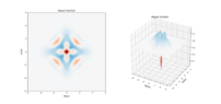
Step 2 - Start in the Ground State
$$ \vert \Psi_i \rangle = \vert 0 \rangle \otimes \vert g \rangle$$
I expect the state looks like
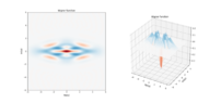
 Step 3 - From Ground State to the Superposition of ground and excited states by applying a drive pulse
$$\vert \Psi \rangle = \frac{1}{\sqrt{2}}\vert 0 \rangle \otimes [\vert g \rangle + \vert e \rangle ] $$
I expect the state looks like

Hamiltonian in array-based form
$$H = H_0 + V + H_D$$
$$H_0 = \hbar \omega_\mathrm{C} \left( a^\dagger a + \frac{1}{2}\right) + \frac{1}{2} \hbar \omega_\mathrm{Q} \sigma_\mathrm{z}$$
$$V_\mathrm{DISP} = \hbar \chi \left( a^\dagger a + \frac{1}{2} \right) \sigma_\mathrm{z}$$
$$\chi = \frac{g^2}{\Delta} \approx 2\pi*(2-10MHz) >> \Gamma $$
$$H_\mathrm{D} = \frac{1}{2} \left[ \sigma_- \tilde{d}(t) + \sigma_+ \tilde{d}^*(t) \right]$$
where ##\tilde{d}(t) = \mathrm{e}^{\mathrm{i}\left( \omega_\mathrm{D} t + \phi \right)}##.
this approximation is that the resonance frequency of the cavity depends on the state of the qubit. We can rewrite the hamiltonian as:
$$H = \hbar \left( \omega_\mathrm{C} + \chi \sigma_\mathrm{z} \right) \left( n + \frac{1}{2}\right) + \frac{1}{2} \hbar \omega_\mathrm{Q} \sigma_\mathrm{z} + H_\mathrm{D}$$
where we see that the resonance frequency of the cavity becomes ##\omega_\mathrm{C} - \chi## when the qubit is in ##\left| \mathrm{g} \right>##, and ##\omega_\mathrm{C} + \chi## when the qubit is in ##\left| \mathrm{e} \right>##. Thus we can measure the resonance frequency of the cavity to know the state of the qubit, without actually measuring the qubit!
Conversely, we can rewrite the hamiltonian as:
$$H = \hbar \omega_\mathrm{C} \left( n + \frac{1}{2}\right) + \frac{1}{2} \hbar \left( \omega_\mathrm{Q} + \chi + 2 n \chi \right) \sigma_\mathrm{z} + H_D$$
where we see that the transition frequency of the qubit is shifted to ##\omega_\mathrm{Q} + \chi## when there are no photons in the cavity (Lamb shift), and additionally for every photon in the cavity the transition frequency is shifted by an additional ##2 \chi## (ac-Stark shift). We can use this phenomenon to accurately measure the number of photons in the cavity by looking at the qubit spectrum.
List of Operators
Time Array
Drive
For a drive term of the form
$$d(t) = A \cos\left( \omega_\mathrm{D} t + \phi \right) = \frac{A}{2} \left[ \mathrm{e}^{\mathrm{i}\left( \omega_\mathrm{D} t + \phi \right)} + \mathrm{e}^{-\mathrm{i}\left( \omega_\mathrm{D} t + \phi \right)} \right]$$
we can invoke the rotating-wave approximation (with the usual caveats) and drop the fast-rotating terms at ##\pm\left(\omega_\mathrm{D}+\omega_\mathrm{Q}\right)##:
$$H_\mathrm{D} = \frac{1}{2} \left[ \sigma_- \tilde{d}(t) + \sigma_+ \tilde{d}^*(t) \right]$$
where ##\tilde{d}(t) = \mathrm{e}^{\mathrm{i}\left( \omega_\mathrm{D} t + \phi \right)}##.
We need to first apply a ##\pi/2## pulse to the qubit to put it int the state $$\vert x \rangle = \frac{1}{2}[\vert g \rangle + \vert e \rangle]$$
Then apply a drive tone to the cavity at frequency ##\omega_c##
Hamiltonian
Solve Schrodinger Equation (without dissipation)
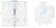
Wigner Function
The Wigner function allows us to see a representation of the state of the cavity in phase space.
We can use the Wigner function to generate probability distributions: the probability distribution of finding the cavity at position ##x## is
$$\left|\psi(x)\right|^2 = \int_{-\infty}^{+\infty} W\left(x,p\right)\mathrm{d}p$$
and similarly at momentum ##p##
$$\left|\psi(p)\right|^2 = \int_{-\infty}^{+\infty} W\left(x,p\right)\mathrm{x}p$$
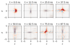
By looking at the Wigner function, we expect to see the Gaussian blob to start at (0, 0), and spiral outwards towards larger amplitudes while rotating around the origin. Below we plot the Wigner function every 20th timestep, *i.e.* with a rate equal to the drive frequency. Thus, we don't see the spiralling but only the Gaussian moving towards larger values of ##x## monotonically.

Plot in 3d to see how the states looks like, which is exactly the same as the demo one. So I believe I transform it correctly to the superposition state.

That's great! I got the state I expected from the demo. However, I got stuck afterwards.
Step 4 - From Superposition to the cavity in a coherent state by applying a drive pulse (it is where I stopped)
$$\vert \Psi \rangle = \frac{1}{\sqrt{2}} [ \vert 2\alpha \rangle \otimes \vert g \rangle + \vert 0 \rangle \otimes \vert e \rangle] $$
I expect the state looks like

I know I need to apply a drive tone to the cavity at frequency ##\omega_c##, to displace the cavity state from ##\vert 0 \rangle## to ##\vert \alpha \rangle##. if and only if the qubit is in the ground state. If the qubit is in the excited state, the cavity remains in the vacuum state.
But I do not know how to apply the drive pulse to state, as they are in tensor product. How can the drive pulse only act on the cavity but not the qubit?
I hope someone can shed some light here.
Hello everyone, I am trying to create cat states in strong dispersive limit for a cavity coupled to a two-level system.
I am attempting to work on it, but I get stuck in step 4-6. I hope someone could help me out.
Here are my references:
1. S. M. Girvin, Schrodinger Cat States in Circuit QED, arXiv:1710.03179
2. Notes
In order to understand my questions, I believe it is good to run the codes with me in jupyter notebook.
(Or if you feel my first thread is too long, please feel free to jump to the second thread that I cannot plot the state I want by visualising Wigner Function)
Installation
Code:
pip install qutipImport Package
Code:
# %matplotlib notebook
import qutip as qt
import numpy as np
import matplotlib.pyplot as plt
from qutip import *
Visualization of Wigner Function:
def plot_wigner_2d_3d(psi):
    #fig, axes = plt.subplots(1, 2, subplot_kw={'projection': '3d'}, figsize=(12, 6))
    fig = plt.figure(figsize=(17, 8))

    ax = fig.add_subplot(1, 2, 1)
    plot_wigner(psi, fig=fig, ax=ax, alpha_max=6);

    ax = fig.add_subplot(1, 2, 2, projection='3d')
    plot_wigner(psi, fig=fig, ax=ax, projection='3d', alpha_max=6);

    plt.close(fig)
    return fig
My Introduction to interpret this case (I am not sure about my Hamiltonian, driving force, etc)
Consider a bipartite system: a cavity is coupled to a two-level system in the strong dispersive limit region.
##\omega_q## denotes the cavity frequency.
##\omega_c## denotes the qubit transition frequency.
g is the vacuum Rabi atom-photon coupling in the cavity
Strong coupling refers to the coupling ##g## between cavity and qubit being larger than the dissipation rates (or line-width) ##\kappa## (cavity) and ##\gamma## (qubit), respectively. The cavity and qubit undergo multiple vacuum Rabi oscillation prior to decacy.
$$g >> \Gamma = max[\gamma, \kappa, 1/T]$$
T is the transit time for the atoms passing through the cavity.
Dispersive refers to the qubit-cavity detuning between the atomic transition and the cavity frequency.
$$\Delta = \omega_\mathrm{C} - \omega_\mathrm{Q} >> g$$
Becasue of the mistach in frequencies, the qubit can only virtually exchange energy with the cavity and the vacuum Rabi coupling can be treated in second-order perturbation theory.
In such limit, we can perform a further approximation of the original Jaynes-Cummings hamiltonian and reach the dispersive hamiltonian \[see Eq. (3.333) from Girvin's notes\]:
(Interaction Hamiltonian ##V_\mathrm{JC}## is the Jaynes-Cummings term \[see Eq. (3.316) from Girvin's notes\])
$$H = H_0 + V + H_D$$
$$H_0 = \hbar \omega_\mathrm{C} \left( a^\dagger a + \frac{1}{2}\right) + \frac{1}{2} \hbar \omega_\mathrm{Q} \sigma_\mathrm{z}$$
$$V_\mathrm{DISP} = \hbar \chi \left( a^\dagger a + \frac{1}{2} \right) \sigma_\mathrm{z}$$
$$\chi = \frac{g^2}{\Delta}2234567890 \approx 2\pi*(2-10MHz) >> \Gamma $$
which is the the effective second-order coupling, *dispersive shift*.
In the dispersive regime, the qubit acts like a dielectric whose dielectric constant depends on the state of the qubit. This causes the cavity frequency to depend on the state of the qubit.
When the qubit is in the excited state, the cavity frequency shifts by ##-\chi##. The disperse shift can be used to read out the state of the qubit. So we can find the qubit state by measuring the cavity frequency by reflecting the microwaves from it and measuring the phase shift of the signal. Because of the frequency difference between cavity and qubit, the photon readout do not excite or de-excite the qubit and the operation is non-destructive.
The dispersive term commutes with both cavity photon number and qubit excitation number. It is doubly QND and can be utilised to make quantum non-demolition measurements of the cavity (using the qubit) and the qubit (using the cavity). It is possible to have QND measurements of photon number and its parity without learning the value of the photon number.
$$H_\mathrm{D} = d(t) \sigma_\mathrm{x}$$
where ##d(t)## is a time-dependent drive term.
In order for the qubit to be dependent on the number of photons in the cavity, the cavity dissipation should needs to be much smaller than the corrections of the qubit resonance frequency
In the simulations we'll set ##\hbar## to one, and neglect the constant term.
##\omega_c## stands for the cavity frequency, ##\omega_q## is the qubit frequency. ##g## is the coupling strength between the cavity and the qubits.
Solving Lindblad Master Equation: with damping (haven't added it to the system, and I do not know if it is necessary)
$$ \dot{\rho} = -\frac{\mathrm{i}}{\hbar} \left[H, \rho\right] + \sum_n \left[ 2C_n\rho C_n^\dagger - \left\{ C_n^\dagger C_n, \rho\right\}\right]$$
where the collapse operators (Lindblad operators) ##C_n## represent the coupling of the system to the environment. A brief introduction can be found on the QuTiP documentation on the [Lindblad Master Equation Solver](http://qutip.org/docs/latest/guide/dynamics/dynamics-master.html).
In our case, the coupling of the harmonic oscillator and two-level system to the environment is represented by ##C=\sqrt{\kappa}a + \sqrt{\gamma}a##, where ##a## is the destruction/annihilation operator (we lose one photon), and $\kappa$ is the photon-loss rate in cavity and ##\gamma## is the photon-loss rate in qubit two-level system.
We'll add a rate of photon loss both on the cavity ##\kappa## and on the qubit ##\gamma##. Since the energy flips between the two parts of the systems, they overall energy-loss rate will be the average of the two rates ##\frac{1}{2}\left(\kappa+\gamma\right)##.
Step 1 - Setting up Parameters
Code:
# Parameters
N = 30  # Hilbert-space cutoff, ideally infinite, but infinite is big
wc = 2 * np.pi * 6.0  # cavity frequency, Grad/s
wq = 2 * np.pi * 5.0  # qubit frequency, same as cavity
#Add dissipation
kappa = 2 * np.pi * 0.001  # cavity linewidth, Grad/s (rate of photon loss)
gamma = 2 * np.pi * 0.005  # qubit linewidth, Grad/s (rate of photon loss)
g = 2 * np.pi * 0.10  # strong coupling strength, Grad/s
delta = abs(wq - wc)  # detuning, GHz
chi = g**2 / delta  # dispersive shift, GHz
T0 = round(abs(2 * np.pi / chi))
USE_RWA = True
Step 2 - Start in the Ground State
$$ \vert \Psi_i \rangle = \vert 0 \rangle \otimes \vert g \rangle$$
Code:
# Initial state: cavity in ground and qubit in excited
# note that qt.basis(2, 1) is ground and qt.basis(2, 0) is excited
psi1 = qt.tensor(qt.basis(N, 0), qt.basis(2, 1))
#print(psi1)
I expect the state looks like
Code:
psi1_demo = qt.tensor(qt.basis(N, 0), qt.basis(2, 1))
plot_wigner_2d_3d(psi1_demo)$$\vert \Psi \rangle = \frac{1}{\sqrt{2}}\vert 0 \rangle \otimes [\vert g \rangle + \vert e \rangle ] $$
I expect the state looks like
Code:
# psi2_demo = tensor(basis(N,0), ((basis(2, 1) + basis(2, 0)) / np.sqrt(2) ))
#print(psi2)
# plot_wigner_2d_3d(psi2_demo)
Hamiltonian in array-based form
$$H = H_0 + V + H_D$$
$$H_0 = \hbar \omega_\mathrm{C} \left( a^\dagger a + \frac{1}{2}\right) + \frac{1}{2} \hbar \omega_\mathrm{Q} \sigma_\mathrm{z}$$
$$V_\mathrm{DISP} = \hbar \chi \left( a^\dagger a + \frac{1}{2} \right) \sigma_\mathrm{z}$$
$$\chi = \frac{g^2}{\Delta} \approx 2\pi*(2-10MHz) >> \Gamma $$
$$H_\mathrm{D} = \frac{1}{2} \left[ \sigma_- \tilde{d}(t) + \sigma_+ \tilde{d}^*(t) \right]$$
where ##\tilde{d}(t) = \mathrm{e}^{\mathrm{i}\left( \omega_\mathrm{D} t + \phi \right)}##.
this approximation is that the resonance frequency of the cavity depends on the state of the qubit. We can rewrite the hamiltonian as:
$$H = \hbar \left( \omega_\mathrm{C} + \chi \sigma_\mathrm{z} \right) \left( n + \frac{1}{2}\right) + \frac{1}{2} \hbar \omega_\mathrm{Q} \sigma_\mathrm{z} + H_\mathrm{D}$$
where we see that the resonance frequency of the cavity becomes ##\omega_\mathrm{C} - \chi## when the qubit is in ##\left| \mathrm{g} \right>##, and ##\omega_\mathrm{C} + \chi## when the qubit is in ##\left| \mathrm{e} \right>##. Thus we can measure the resonance frequency of the cavity to know the state of the qubit, without actually measuring the qubit!
Conversely, we can rewrite the hamiltonian as:
$$H = \hbar \omega_\mathrm{C} \left( n + \frac{1}{2}\right) + \frac{1}{2} \hbar \left( \omega_\mathrm{Q} + \chi + 2 n \chi \right) \sigma_\mathrm{z} + H_D$$
where we see that the transition frequency of the qubit is shifted to ##\omega_\mathrm{Q} + \chi## when there are no photons in the cavity (Lamb shift), and additionally for every photon in the cavity the transition frequency is shifted by an additional ##2 \chi## (ac-Stark shift). We can use this phenomenon to accurately measure the number of photons in the cavity by looking at the qubit spectrum.
List of Operators
Code:
# Cavity operators
a = qt.tensor(qt.destroy(N), qt.qeye(2))  # annihilation
n = a.dag() * a  # photon number
x = qt.tensor(qt.position(N), qt.qeye(2))  # x = 1/sqrt(2) * (a + a.dag())
p = qt.tensor(qt.momentum(N), qt.qeye(2))  # p = -1j/sqrt(2) * (a - a.dag())
# with these definitions: <x>^2 / 2 + <p>^2 / 2 = <n>
# Qubit operators (Pauli matrices)
sx = qt.tensor(qt.qeye(N), qt.sigmax())  # sp + sm
sy = qt.tensor(qt.qeye(N), qt.sigmay())  # 1j * (sm - sp)
sz = qt.tensor(qt.qeye(N), qt.sigmaz())
sp = qt.tensor(qt.qeye(N), qt.sigmap())  # (sx + 1j * sy) / 2 == sm.dag()
sm = qt.tensor(qt.qeye(N), qt.sigmam())  # (sx - 1j * sy) / 2 == sp.dag()
# identity matrix
eye = qt.tensor(qt.qeye(N), qt.qeye(2))
#collapse operator
c_ops = [
    np.sqrt(kappa) * a,
    np.sqrt(gamma) * sm,
]
Time Array
Code:
# Time array
fs = 120.0  # sampling frequency, GHz
dt = 1 / fs
T = 2 * T0  # time, ns
ns = int(round(fs * T))  # nr of samples
tlist = dt * np.arange(ns)  # nanoseconds
Drive
For a drive term of the form
$$d(t) = A \cos\left( \omega_\mathrm{D} t + \phi \right) = \frac{A}{2} \left[ \mathrm{e}^{\mathrm{i}\left( \omega_\mathrm{D} t + \phi \right)} + \mathrm{e}^{-\mathrm{i}\left( \omega_\mathrm{D} t + \phi \right)} \right]$$
we can invoke the rotating-wave approximation (with the usual caveats) and drop the fast-rotating terms at ##\pm\left(\omega_\mathrm{D}+\omega_\mathrm{Q}\right)##:
$$H_\mathrm{D} = \frac{1}{2} \left[ \sigma_- \tilde{d}(t) + \sigma_+ \tilde{d}^*(t) \right]$$
where ##\tilde{d}(t) = \mathrm{e}^{\mathrm{i}\left( \omega_\mathrm{D} t + \phi \right)}##.
We need to first apply a ##\pi/2## pulse to the qubit to put it int the state $$\vert x \rangle = \frac{1}{2}[\vert g \rangle + \vert e \rangle]$$
Then apply a drive tone to the cavity at frequency ##\omega_c##
Code:
# Drive
wd = wq  # drive at the qubit transition frequency
amp = np.pi
phase = -np.pi / 2
if USE_RWA:
    drive = amp * np.exp(1j * (wd * tlist + phase))
else:
    drive = amp * np.cos(wd * tlist + phase)
# Drive
#wd = wc  # drive at resonance
#amp = 10.0
#phase = -np.pi / 2
#if USE_RWA:
#    drive = amp * np.exp(1j * (wd * tlist + phase))
#else:
#    drive = amp * np.cos(wd * tlist + phase)
# Cavity drive
#wd_c = wc - chi  # drive at the frequency corresponding to ground state
#amp_c = 0.04
#phase_c = np.pi / 2
#drive_c = amp_c * np.sin(np.pi / T * tlist)**2 * np.exp(1j * (wd_c * tlist + phase_c))
Hamiltonian
Code:
H0 = H0 = wc * (a.dag() * a + eye / 2) + 0.5 * wq * sz
V = chi * (a.dag() * a + eye / 2) * sz  # dispersive hamiltonian
H = [
    H0,
    V,
    [sm, 0.5 * drive],
    [sp, 0.5 * drive.conj()],
]
#H = [
#    H0,
#    V,
#    [a, 0.5 * drive_c],
#    [a.dag(), 0.5 * drive_c.conj()],
#]
Solve Schrodinger Equation (without dissipation)
Code:
output = qt.sesolve(H, psi1, tlist)Wigner Function
The Wigner function allows us to see a representation of the state of the cavity in phase space.
We can use the Wigner function to generate probability distributions: the probability distribution of finding the cavity at position ##x## is
$$\left|\psi(x)\right|^2 = \int_{-\infty}^{+\infty} W\left(x,p\right)\mathrm{d}p$$
and similarly at momentum ##p##
$$\left|\psi(p)\right|^2 = \int_{-\infty}^{+\infty} W\left(x,p\right)\mathrm{x}p$$
By looking at the Wigner function, we expect to see the Gaussian blob to start at (0, 0), and spiral outwards towards larger amplitudes while rotating around the origin. Below we plot the Wigner function every 20th timestep, *i.e.* with a rate equal to the drive frequency. Thus, we don't see the spiralling but only the Gaussian moving towards larger values of ##x## monotonically.
Code:
fig2, ax2 = plt.subplots(2, 4, sharex=True, sharey=True)
ax2 = ax2.flatten()
xvec = np.linspace(-5, 5, 200)
for axi, idx in enumerate(range(0, ns // 2, ns // 16)):
    rho = output.states[idx]
    W = qt.wigner(rho, xvec, xvec)
    wlim = np.abs(W).max()
    ax2[axi].imshow(
        W, cmap='RdBu_r', vmin=-wlim, vmax=wlim, origin="lower",
        extent=(xvec.min(), xvec.max(), xvec.min(), xvec.max()),
    )
    ax2[axi].axhline(0.0, c="tab:gray", alpha=0.25)
    ax2[axi].axvline(0.0, c="tab:gray", alpha=0.25)
    ax2[axi].set_title(f"t = {tlist[idx]} ns")
[ax2[axi].set_xlabel(r"$x$") for axi in [4, 5, 6, 7]]
[ax2[axi].set_ylabel(r"$p$") for axi in [0, 4]]
Plot in 3d to see how the states looks like, which is exactly the same as the demo one. So I believe I transform it correctly to the superposition state.
Code:
psi2 = rho
plot_wigner_2d_3d(psi2)
That's great! I got the state I expected from the demo. However, I got stuck afterwards.
Step 4 - From Superposition to the cavity in a coherent state by applying a drive pulse (it is where I stopped)
$$\vert \Psi \rangle = \frac{1}{\sqrt{2}} [ \vert 2\alpha \rangle \otimes \vert g \rangle + \vert 0 \rangle \otimes \vert e \rangle] $$
I expect the state looks like
I know I need to apply a drive tone to the cavity at frequency ##\omega_c##, to displace the cavity state from ##\vert 0 \rangle## to ##\vert \alpha \rangle##. if and only if the qubit is in the ground state. If the qubit is in the excited state, the cavity remains in the vacuum state.
But I do not know how to apply the drive pulse to state, as they are in tensor product. How can the drive pulse only act on the cavity but not the qubit?
I hope someone can shed some light here.
Attachments
Last edited by a moderator: