Runge-Kutta 4 w/ some sugar on the top: How to do error approximation?

[BvU]

Coming back to

I've now changed it to 0.00005. ##\mathcal O## is 0.5⋅10−6, which is the highest error tolerated by the assignment.

and

"The answers should have at least 6-8 correct digits, somewhat depending on question" (yes, this is what the assignment says)

when you report

x-values for comparison for fun, here's what I get using the initial conditions given in the top post: (for the three bounces before x=1.2)

-3.53496e-01 4.3385e-01 9.1342e-01

Where I'm afraid I have to remark that this doesn't satisfy the 'at least 6-8 correct digits' ...

(and the ##\mathcal O## is also on edge -- I personally would take 0.5E-7 or even 0.5E-8 ...

- - - -

When I finally got something to work (see #18) the results allow guestimating the 'correct digits':

(step size, ##x_0## for bounce 1,2,3)

5.0e-5 ##\qquad## -0.353496957103320 ##\qquad## 0.433854331752568 ##\qquad## 0.913422978195822

5.0e-4 ##\qquad## -0.353496957103362 ##\qquad## 0.433854331752487 ##\qquad## 0.913422978195706

5.0e-3 ##\qquad## -0.353496957539166 ##\qquad## 0.433854330903075 ##\qquad## 0.913422976982109

2.5e-2 ##\qquad## -0.353497244187681 ##\qquad## 0.433853767233959 ##\qquad## 0.913422170776847

So a step size of 5e-3 looks like a safe choice with 8⁺ significant digits.

- - - - -

Step size 5e-4 gave me local truncation errors of machine precision (#32), so I tried again with step size 5e-3.
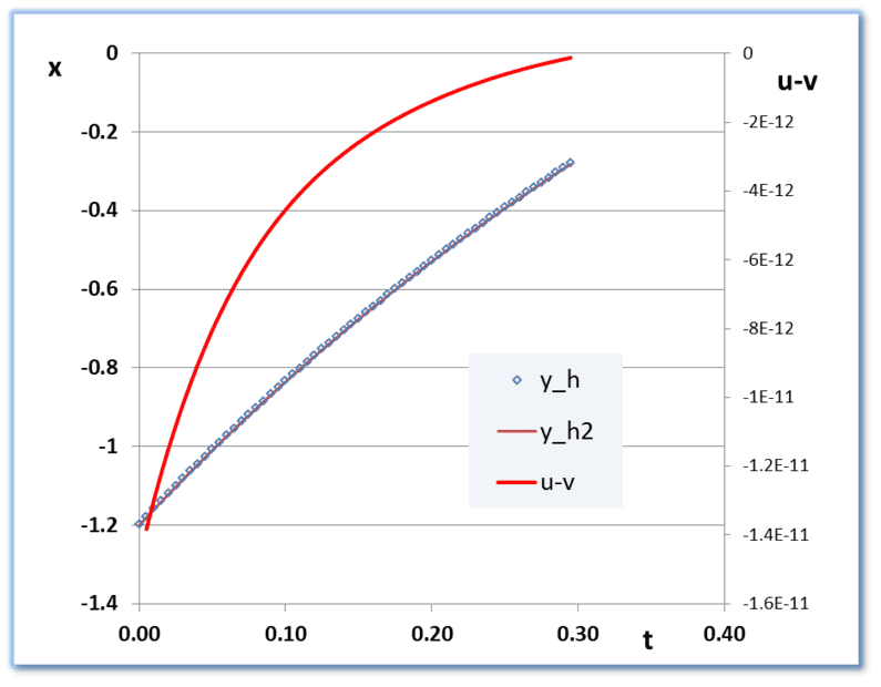
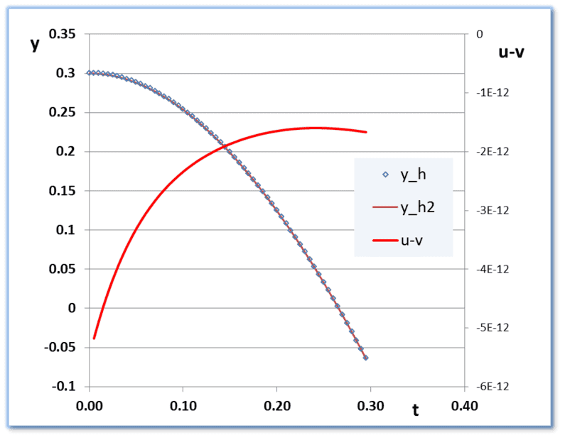
Forget about the bouncing, just integrate from 0 to t=0.3 in 60 steps.

What y do you compare to do that? And how do you find out where in the "solution" matrix the new y is stored?

Gives me 61 vectors ##(t_n,x_n,y_n,\dot x_n, \dot y_n)\quad ## n = 0 to 60

At each of these points ##n## I also do a two step RK4 with step size 2.5e-3.
That gives me a vector ##(t_{n+1},x^*,y^*,\dot x^*, \dot y^*)\quad ##

So I have (in MIT (7.17 notation) ##y(x+h)## and ##y(x+h/2+h/2)##.
And therefore an estimate of the local truncation error for both horizontal position: ##x_{n+1} - x^*## and vertical position: ##y_{n+1} - y^*##.
In pictures:

x(t) is almost a straight line and y(t) is almost a parabola .
The red lines show the local truncation error estimates (I dubbed them 'u-v' somehow) All negative.
Even a pessimistic global error estimate (just add absolute values) yields a maximum uncertainty in ##x## and ##y## after 54 steps of
about 2e-10. Consistent with the 9 significant digits above.

With the bouncing back in: two or three steps to find the exact moment are enough; the accumulated error for the first bounce will still be 2e-10 and the second and third a bit more. But no reason at all to halve step sizes.

I can't answer 'where in the "solution" matrix the new y is stored?'
In the fortran I added an array for the ##+h/2+h/2## results. In your matlab that would be a second solution matrix, I suppose.

I see pbuk added two posts. Will look at them later.

##\ ##

 

[bremenfallturm]

t=nh0=10nh1. And because you are using a sufficiently small step size, the two values are similar to around machine epsilon - the difference in the values is your error estimate.

Ah - so it's really just that simple? Wow, I've overcomplicated this for sure!

* Stoer and Bulirsch's book Introduction to Numerical Analysis was at one time the standard text for an introductory course in numerical analysis: you might find the first chapter on error analysis particularly helpful.

Thank you so much for the tip. I realize I'm lacking some fundamentals and I will definitely give it a read. I love how it starts with error analysis! I have been using Sauer's book, whatever it is called. I'm a first year student so I'm still learning how to read academic material, but let's just say I've been looking for a good book in numerical analysis.

With the bouncing back in: two or three steps to find the exact moment are enough; the accumulated error for the first bounce will still be 2e-10 and the second and third a bit more. But no reason at all to halve step sizes.

You're indeed correct, using the error calculation suggested by pbuk, I got a relative error of 2e-10 which came out really quickly!

Now I'm struggling a little with how the next part of the assignment:
I'm sorry if this is out of scope of the original question, but we've come such a long way here. And hey, also want to stop for a minute and say a massive thank you! While the error calculation turned out really simple, as you can tell I was not aware how to do it at first.

Anyways, I'm talking about this part:

2. If the ball is launced with y˙=0 with one bounce before the net, what initial values of x˙ will make the ball be at net height y=0.12 where x=0, assuming the table is centered around x=0.
3. Find a starting angle given that |v|=10 so that the ball is at y=0 when x=1.2. Also find the time where the ball is at x≤1.2 for that value.

Alright, so the problem here is that my current method is to simply use the bisection method for both of these problems to solve for the equation ##f(x, \dot x, y, \dot y)=0## (Eqn. 1) in question 3 and ##0.3-f(x, \dot x, y, \dot y)=0## (Eqn.2) in question 2, where what ##f## gives as the output is the value at ##x=a##, where ##a## is the ##x## value we want Eqn. 1 or Eqn. 2 to be satisfied in depending on question. I'm using ##h=0.5e-2##.
To get the return value of ##f##, here is what I do:
Now, I tried two things for step 1:
1.1 Run Runge-Kutta 4 until the error tolerance criteria is achieved using starting guesses ##(x, \dot x, y, \dot y)##, ##x=-1.2## and ##y=0.3## for both of the question, and ##\dot y = 0## for question 3 additionally.
and:
1.2 Run Runge-Kutta 4 (just like 1.1) with the exception that I *do not* check for errors:
The question I will ask below is about 1.1 and 1.2, but if you're interested, here is what I'm doing to get the return value of ##f## after that:

Spoiler: More algorithms!

2. Interpolate near the point that we're looking for - in question 3. we want to check ##x=1.2## and similarly in question 2, we want to check ##x=0##.
3. Return the value that the interpolation polynomial gives at exactly the point that I've previously called ##x=a## (called "the point we're looking for" in 2.)
4. Repeat until (Eqn. 1)or (Eqn. 2) depedning on problem is close to ##0## with a relative error tolerance (for the secant method) of ##\mathcal O=0.5e-6##.

For example, if I try to solve question 2. with starting guesses ##x_1=4##, ##x_2=5##, I getf or the first 3 iterations:

iteration	y value at x=0 (want y=0) (using method 1.1)	y value at x=0 (want y=0) (using method 1.2)
1	-1.347990e-02	-1.347993e-02
2	-2.706809e-02	-2.436346-04
3	5.1092449e-03	-2.706811e-02
...

Method 1.1 is horribly sluggish: The code overall takes about 3 minutes to run. That's really slow. I don't know what's to be expected, but given that my code for question 1. (nowadays) run in less than a second, I'm not a fan of what's currently happening. Same pattern on question 3, it takes forever to run.

However, here is actually my main question: If I use Method 1.2, i.e. no error tolerance on Runge-Kutta, it takes about half a minute or so to run. I get, for question 2., the solutions:
##x_1=4.855930097130874##
##x_2=2.926130865384258##
(just copied all digits MATLAB gave me - I know not all are perfect!)

Recall that method 1.2 did not use any error tolerance when solving the actual equation. However, if I plug ##x_1## and ##x_2## into Runge-Kutta 4, now with an error tolerance of ##0.5e-6##. I get:
##y_{at x=0}(x_1)=1.200001965196033e-01##
##y_{at x=0}(x_2)=1.199999999181511e-01##
which looks really good to me. The relative error works out nicely to be ##3.66157e-10## for ##x_2## and close to machine precision for ##x_1##.

Aka. I think it's safe to not use an error boundary when I am solving for ##x_1## and ##x_2##. Does this sound reasonable? This turned out to be a lot of text, hope I didn't lose anyone somewhere!

Footnote: same story for question 3!

 

[pbuk]

I don't have time to read all of that at the moment, but I have two observations:

Method 1.1 is horribly sluggish: The code overall takes about 3 minutes to run. That's really slow. I don't know what's to be expected, but given that my code for question 1. (nowadays) run in less than a second, I'm not a fan of what's currently happening. Same pattern on question 3, it takes forever to run.

I guess you are using the bisection method to goal seek, running the integration each time as I suggested in #35?

You have 54 bits of precision so if the routine takes less than a second you should be there in less than a minute. Three minutes is not a great deal different - I suspect the difference may be due to MATLAB doing a lot of memory management due do storing a mass of useless intermediate results in vectors. I would write this in a procedural language (Python, Java, C++, maybe even Node JS) which would need less than 1 KB storage but I appreciate you don't have the choice.

Aka. I think it's safe to not use an error boundary when I am solving for ##x_1## and ##x_2##. Does this sound reasonable? This turned out to be a lot of text, hope I didn't lose anyone somewhere!

Yes, the smoothness of the solution is pretty much the same for all relevant initial conditions so once you have determined the global error for a given step size you don't need to keep checking it. Probably worth doing one final confirmation once you have found a solution though, again as I suggested in #35.

 

[bremenfallturm]

I guess you are using the bisection method to goal seek, running the integration each time as I suggested in #35?

Ah sorry - I am still using interpolation. Haven't implemented your method.

I need to get back on quesion 3 - looks like it might not be sufficient to solve without an error tolerance.

 

[BvU]

Just showing off . Don't have MatLab, so downloaded Octave and fought my way in. Both horrible and fascinating at the same time (for a 1980's Fortran 77 'expert'). Results identical to what I already had in all digits -- including the error estimates and the bouncing points
( -0.35349695753917 ##\qquad## 0.43385433090308 ##\qquad## 0.91342297698211 )

Infinite hassle to wrap a program into a subroutine and other Octave/MatLab ideosyncracies now stop me from moving forward. Temporarily, I hope .


Just so I understand parts 2 and 3: Isn't it enough for part 2 to insert a small step backwards when ##y## falls below 0.12 -- in the same way as is done when y falls below 0 to find the bouncing points ? And then when this ##x_{y=0.12}## is added to/subtracted from -1.2 2 is done?
And in 3 you want the second bounce at ##x=1.2##, right ? (haven't played that game for ages...)

##\ ##

 

[bremenfallturm]

Isn't it enough for part 2 to insert a small step backwards when y falls below 0.12 -- in the same way as is done when y falls below 0 to find the bouncing points ?

Yes, that's technically right. Currently I calculate with Runge-Kutta 4 until ##x>0## and then interpolate near ##x=0## to find the value at ##y=0##. This gives me a solution that's basically perfect

And in 3 you want the second bounce at x=1.2, right ? (haven't played that game for ages...)

Yes! That's correct!

I think I've solved these steps by myself - I will update and write up a longer thank-you post when I've looked through the last things!

 

[BvU]

Yes! That's correct!

With v=10 that means serving (at -1.2m, 0.3 m) in a direction about -50 degrees so it will bounce up one meter . Am I missing something ?

##\ ##

 

[bremenfallturm]

With v=10 that means serving (at -1.2m, 0.3 m) in a direction about -50 degrees so it will bounce up one meter . Am I missing something ?
View attachment 344085
##\ ##

That's what I got as well. According to the solution, apparently there is supposed to be two valid bounces. Can't understand why. Do they mean that "illegal serves" are ok for the angles? Do you have any clue?

 

[BvU]

According to the solution, apparently there is supposed to be two valid bounces. Can't understand why. Do they mean that "illegal serves" are ok for the angles?

Do they tell you the answer ?

Do you have any clue?

I'm lost. If you can only vary the angle there is only one angle that lets the second bounce end op at 1.2 m.
(serving with a positive angle with the condition that the first bounce is before the net means the second bounce is well short of 1.2 m)

##\ ##

 

[bremenfallturm]

Do they tell you the answer ?

Oral feedback, they don't give values or anything sadly.

I'm lost.

Me too. I guess if anyone complains about my solution I'll argue why it's wrong.

Quick extra question, if you don't mind, I tried using this technique, see the quoted post for more context if you don't remember

To directly translate this method from what we call it in my language would be "distrubance counting". I've been trying to find the English name for months, haha!
The principle is. Let's say you have a function f(x,y,z) where x,y,z have insecurities ±1 as an example What you do is, try each combination: f(x⋅1.01,y,z), f(x,y⋅1.01,z), ...,
f(x⋅0.99,y,z), ..., f(x⋅1.01,y⋅1.01,z), and so on.
If you compare the differences from f(x,y,z) for each value, an estimate of the global error is

Let's say I vary the constant ##k_x## for example, s.t. ##k_{x1}=k_x\cdot 1.01##
My original values are

−0,3534969571 (1st bounce)

0,4338543317 (2nd bounce)

0,1835159822 (y @ x=0)

with the perturbation I get

-0,3552185576 (1st bounce)

0,4283719732 (2nd bounce)

0,18419183595 (y @ x = 0)

I see that the implies that at most the difference is at the order of ##10^{-1}##, i.e. the tabular error that is introduced means that the uncertainty will be much bigger. Again, this is a little out of the sope of this topic, but does this seem reasonable? It feels like it is a lot worse than those 8 digits, but I understand that distrubing a system can impact it significantly.

 

[pbuk]

I see that the implies that at most the difference is at the order of ##10^{-1}##, i.e. the tabular error that is introduced means that the uncertainty will be much bigger.

I don't see that: the greatest difference in the results for a 1% change in this input is ## \frac {0,4338543317}{0,4283719732} \approx 1.3\% ##, so this system is not particularly sensitive to parameters.

I understand that distrubing a system can impact it significantly.

Such systems of ODEs are often referred to as stiff (although strictly speaking this only applies to a subset of these). I expect you will come across these and methods that are suitable to solve them later in your course.

 

[pbuk]

If you can only vary the angle there is only one angle that lets the second bounce end op at 1.2 m.

Really? Similar problems often have two solutions: a high, slow 'lob' (which you have found) and a low, fast 'chip' - but I can see that the constraints of the first bounce and clearing the net may prevent this here.

 

[BvU]

Really? Similar problems often have two solutions: a high, slow 'lob' (which you have found) and a low, fast 'chip' - but I can see that the constraints of the first bounce and clearing the net may prevent this here.

The initial condition for the position where the serve occurs appears to block a second solution

 

[bremenfallturm]

don't see that: the greatest difference in the results for a 1% change in this input

Heh you're right, my bad. Should have looked at the relative error.
Now I tried to do some more rigourous error analysis using the method I wrote about earlier, i.e. introduce a disturbance of ##\pm 1\%## to each parameter at a time, write down the output, and then take the sum of the maximal errors. Here are (the only) notes my teacher have about it:

"The value without disturbances are ##96## and the sum of the disturbances are ##11##, so we write that the area is ##96\pm 11m^2##" (the function returns area in this example).

The assignment is asking for "safe digits", so a relative error in my case. Here is an example of how I've worked through the first question (the one that just involves solving the differential equation):
Remember it asks for the coordinates of the first two bounces!

Spoiler: Lots of numbers !

	Changed variable	Output	No disturbance	Down (0,99*variable)	Up (1,01*variable)	Difference 1 (no disturbance)-down	Difference 2 (no disturbance)-up	Max (Difference 1, Difference 2)
	m	Bounce_1	−0,3534969571	−0,3547233267	−0,3522913222	0,001226369546	0,001205634921	0,001226369546
	m	Bounce_2	0,4338543317	0,4274372697	0,4402051997	0,006417061984	0,006350868021	0,006417061984
	m	y at x=0	0,1835159822	0,1834884753	0,1835206618	0,00002750689218	0,000004679565103	0,00002750689218
	kx	Bounce_1		−0,3552185576	−0,3447185922	0,001721600478	0,008778364925	0,008778364925
	kx	Bounce_2		0,4283719733	0,4390468016	0,005482358439	0,005192469933	0,005482358439
	kx	y at x=0		0,184191836	0,177648169	0,00067585377	0,005867813141	0,005867813141
	ky	Bounce_1		−0,3529867127	−0,3529867127	0,0005102444411	0,0005102444411	0,0005102444411
	ky	Bounce_2		0,4329749907	0,4329749907	0,0008793410221	0,0008793410221	0,0008793410221
	ky	y at x=0		0,1828156662	0,1828156662	0,0007003159692	0,0007003159692	0,0007003159692
	v_0	Bounce_1		−0,3608115286	−0,3462025429	0,007314571446	0,007294414249	0,007314571446
	v_0	Bounce_2		0,4227798015	0,44486305	0,01107453022	0,01100871829	0,01107453022
	v_0	y at x=0		0,1852609977	0,1816099484	0,001745015489	0,001906033788	0,001906033788
	g	Bounce_1		−0,3498196521	−0,3571245146	0,003677304986	0,003627557502	0,003677304986
	g	Bounce_2		0,4394084953	0,4283665304	0,005554163614	0,005487801335	0,005554163614
	g	y at x=0		0,182575263	0,1844027637	0,000940719193	0,0008867815271	0,000940719193

Sorry in advance for hitting you in the face with a bunch of numbers. The "No disturbance" column of course have the same three values throughout, so I just included them once.

Alright, so now I sum up the everything in the max column for each respective variable.
For example, for bounce 1, I sum up: ##\text{Sum of max errors for bounce 1: } \sum \left\| \Delta \right\| = 0.001226369546 + 0.008778364925 + 0.0005102444411 + 0.007314571446 + 0.003677304986 = 0.02150685534## (what I sum up is marked in bold above)
So now I can calculate the relative error for bounce 1 as ##\text{Relative error for bounce 1: } \frac{\text{sum of max errors}}{\text{real value of bounce 1}} = \left| \frac{0.02150685534}{-0.3534969571} \right| \approx 6.08\%##

This does seem a bit fishy to me, since the relative error ends up becoming quote large when I sum up the maxes like that. I don't quite follow along if I can do it like that (again, I've found no material outside the screenshot I included about this method, and as you understand I've never been properly introduced to error calculation.

 

[bremenfallturm]

Nice work! Just checking, but the '0, 00122...' are typos right?

Hmm, don't see an obvious typo... could you elaborate?

Also, does "nice work" imply that the relative error calculation seems legit?
So as an answer I can say that the uncertainty of bounce 1 occurs at ##−0,3534969571\pm 6,08\%##.

 

[bremenfallturm]

Decimals are written as X.XXX... and not X, XXX... It's just a nit, don't mean to make it a big deal.

Aha, I see what you mean. I copied it from where I have noted the data and it ended up like that. Thanks for pointing it out!

 

[BvU]

The assignment is asking for "safe digits", so a relative error in my case. Here is an example of how I've worked through the first question (the one that just involves solving the differential equation):
Remember it asks for the coordinates of the first two bounces!

The assignment text is confusing me (again). Your 'lots of numbers' and the ##\sum|\Delta|## propagation method give me 6% error in bounce 1, 7% in bounce 2 and 5 in ##y_{x=0}##. Huge ! (and the ##\sqrt {\sum\Delta^2}## about 3.5%, also huge).
Note that the uncertainty in the error estimate is considerable and only seldom warrants giving more than 1.5 digit !
(one digit, two if the first is a 1) .

"The answers should have at least 6-8 correct digits, somewhat depending on question" (yes, this is what the assignment says)
You also need to assume that every given value has an uncertainty of 1%. Use that to approximate the tabular error, and then include that in the calculation of te total error of your program.

So as an answer I can say that the uncertainty of bounce 1 occurs at −0,3534969571 ± 6,08%.

Which comes down to 0.35 ##\pm## 0.02
Two digits, no more.

What's the point of doing a 6-8 correct digits calculation if these uncertainties in the parameters are so big ?

[edit] can you check your 'lots of numbers' ? I find it strange that the first bounce occurs further to the left if ##k_x## is lowered ....




##\ ##

 

[bremenfallturm]

What's the point of doing a 6-8 correct digits calculation if these uncertainties in the parameters are so big ?

I see what you mean, it has of course frustrated me a bit too. We're supposed to consider two scenarios: the first one assuming that the input data is perfect (this yields 6-8 safe digits) and the second one assuming that the input data has that ##\pm 1\%## error (this yields 2 safe digits as we both concluded).
I will just assume that they want the first scenario to have the requested accuracy and the second one is separate to show that I have studied how errors affect the assignment.
I think the high requirement for precision is to show that we know how to apply efficient methods and predict errors, though it's not clearly stated which scenario that should have the requested accuracy, only that a "total error estimate" should be included.

 

[pbuk]

I will just assume that they want the first scenario to have the requested accuracy and the second one is separate to show that I have studied how errors affect the assignment.

Yes, this is how I interpret it too.

 

[bremenfallturm]

Thank you guys! So now I'm actually finalizing the thing that the topic title asks about: I'm putting together an answer!
Once again, please forgive me for not knowing these things that probably seem obvious to you. (Reminding you again that I'm a first year student and haven't been properly taught about error approximation!)

So let's say I want to provide an answer to everything.

1. Some answers have more accurate digits (7-9), does it make sense to round all numerical solutions to 6 digits or should I include all of them? (is it good practice to answer with all values having the same number of digits or should I not bother).

2. I am asked for a relative error, does it make sense to indicate the error boundary in percentages like this: $$\pm 0.5\cdot 10^{-6}\%$$?

3. I am also asked to indicate the presentation error. That is the error caused by rouding (for example, the presentation error of ##1,2345## is ##\underbrace{1,2345689}_{\text{non-rounded value}}-1,2345=0,0000689## if I round to 5 digits. Should I take that value, call it ##E_{presentation}## and express it in percentage like ##E_{presentation pct}=\frac{E_{presentation}}{\text{non-rounded value}}##, or should I not bother about expressing it in percentage?

 

[bremenfallturm]

I double-checked my table, looks like you're right. k_x down gives −0,352986712689222.
I have another question. I have from above an uncertainty that is >5%. Doesn't that mean that no digits are safe? Since 0,5e-1 implies once safe digit. What do I answer in that case?

 

[BvU]

I double-checked my table,

Did you ? And did you notice something strange with with ##k_y## too ?

looks like you're right. k_x down gives −0,352986712689222.

I get -0.352986712689222
and for ##k_{x, up}## I get -0.35521856 and not -0.352986712689222

I have another question. I have from above an uncertainty that is >5%. Doesn't that mean that no digits are safe? Since 0,5e-1 implies once safe digit. What do I answer in that case?

We've whittled it down to 4% I think... But even 6% warrants two digits: 0.353 ##\pm## 5% is 0.353 ##\pm## 0.018 (the 1.5 digit if you firmly believe the accuracy if the error) or at worst 0.35 ##\pm## 0.2

And I think adding absolute ##\Delta## is way too pessimistic; adding squares and taking the root is much more sensible.

Also see #52

will look at #55 tomorrow. But ##\pm 0.5\cdot 10^{-6}\%## must be a mistake

##\ ##

 

[bremenfallturm]

Did you ? And did you notice something strange with with ##k_y## too ?


I get -0.352986712689222
and for ##k_{x, up}## I get -0.35521856 and not -0.352986712689222



We've whittled it down to 4% I think... But even 6% warrants two digits: 0.353 ##\pm## 5% is 0.353 ##\pm## 0.018 (the 1.5 digit if you firmly believe the accuracy if the error) or at worst 0.35 ##\pm## 0.2

And I think adding absolute ##\Delta## is way too pessimistic; adding squares and taking the root is much more sensible.

Also see #52

will look at #55 tomorrow. But ##\pm 0.5\cdot 10^{-6}\%## must be a mistake

##\ ##

Aha, I see you. Embarrasing, sorry!
I've always thought that a relative error of ##0.5\cdot10^{-n}## where ##n## is the number implies ##n## safe digits. Is that wrong?
It looks like it's the change in velocity that is causing such huge error.

 

[pbuk]

I've always thought that a relative error of ##0.5\cdot10^{-n}## where ##n## is the number implies ##n## safe digits. Is that wrong?

Yes it is wrong - that is an absolute error.

Edit: it could also be a relative error - see #61.

 

[pbuk]

And I think adding absolute ##\Delta## is way too pessimistic; adding squares and taking the root is much more sensible.

This depends on context - I would be inclined to do both, stating the assumption that must be made in order to use the second approach.

 

[bremenfallturm]

Yes it is wrong - that is an absolute error.

Aha, thank you! So a relative error of ##0.5\cdot 10^{-n}## implies ##n+1## safe digits? According to
https://math.stackexchange.com/ques...-relative-error-give-number-of-correct-digits . (that's good - or at least better - news!)

This depends on context - I would be inclined to do both, stating the assumption that must be made in order to use the second approach.

My lecturer uses ##\sum \left|\Delta \right|## when using the method I described, i.e. not the propagation suggested by BvU. I assume that the course wants me to use that one, even if it is pessimistic.

 

[pbuk]

Aha, thank you! So a relative error of ##0.5\cdot 10^{-n}## implies ##n+1## safe digits? According to
https://math.stackexchange.com/ques...-relative-error-give-number-of-correct-digits . (that's good - or at least better - news!)

Hmmm, there is the danger of confusion here. Let's make sure we are all clear on the definitions:

If the true value of a quantity is ## x ## and the measured value is ## x_0 ## then the absolute error is ## x_0 - x ## and the relative error is ## \frac x{x_0} -1 ##.​

https://mathworld.wolfram.com/AbsoluteError.html
https://mathworld.wolfram.com/RelativeError.html

So ##0.5\times10^{-n}## could be either a relative error or an absolute error.

My lecturer uses ##\sum \left|\Delta \right|## when using the method I described, i.e. not the propagation suggested by BvU. I assume that the course wants me to use that one, even if it is pessimistic.

I agree with your lecturer, and it is not pessimistic: in the absence of other information it is the right method to use. The method suggested by BvU is optimistic because it assumes that the errors are independent random variables and in this problem there is no reason to indicate that that is true - which is why I suggested that if you did use it you should state that assumption.