Order in Renormalization Theory

In summary: In other words, all divergences appearing in renormalization perturbation theory are of order ##\hbar##.
  • #1
taishizhiqiu
63
4
I am currently studying QFT with 'An Introduction to Quantum Field Theory' by peskin. In part 2 (renormalization) of the book, he introduces counterterms and shows how to compute scattering amplitude with them.
Below are counterterms of [itex]\phi^4[/itex] theory:
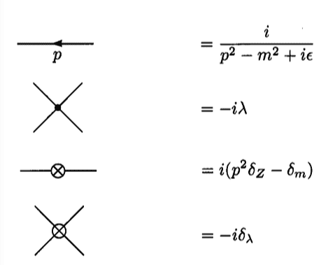
DAE819FC-4B8C-44D9-BBEA-C6CDFF6E859E.png

Then he calculates a 2-2 scattering process to the second order:
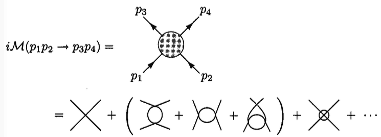
D35F5BE9-A5C2-4F7D-BE2F-957D05B284FE.png

Here I have a few questions:

1. Why the fifth diagram in the second line of the second picture is of the same order to the previous three diagrams?

2. Now that [itex]\delta_m,\delta_Z,\delta_\lambda[/itex] are infinite numbers, how can they use perturbation theory and what is the meaning of order in renormalization perturbation theory?

Edit: should this thread be moved to Homework section? It just cannot be fit into the question structure there.
 
Last edited:
Physics news on Phys.org
  • #2
It's most simple to look at perturbative renormalization in terms of the finite physical quantities. So you start at tree level. There's no counterterm necessary since you just take the S-matrix elements from your Feynman rules, evaluate cross sections at tree level ("Born approximation") and fit the coupling and masses to some experiment.

Then you go further and do a one-loop calculation. Then you'll find divergent loop integrals, but even if you wouldn't have divergences, you'd have to refit your parameters to the experiment again, i.e., you need counter terms in order to readjust the parameters in terms of their physical quantities. At the order given by the Feynman diagrams, both your (divergent) loop diagrams and the corresponding counter terms are of order ##\hbar## (relative to the tree-level order). Then you go on, and do two-loop diagrams. After taking into account the counter terms of the one-loop result for the subdivergences according to Zimmermann's forest formula you are again left with local overall counterterms which cancel the overall divergences of the two-loop diagrams. They are of the same order ##\mathcal{O}(\hbar^2)## as the (divergent) two-loop diagrams and so on. In this iterative way, using Weinberg's convergence theorem and the BPHZ formalism you can show that ##\phi^4## theory is Dyson renormalizable order by order in perturbation theory, i.e., you only need counter terms of the form already present in the bare Lagrangian, i.e., order by order the renormalization of the wave function norm, mass, and coupling constant is sufficient to get finite results for the S-matrix elements entering observable quantities like cross sections.
 
  • #3
vanhees71 said:
At the order given by the Feynman diagrams, both your (divergent) loop diagrams and the corresponding counter terms are of order ##\hbar## (relative to the tree-level order).

Please explain why the one-loop diagram and counterterm diagram showed in my post is of order [itex]\hbar[/itex](especially the counterterm diagram). Most textbooks set [itex]\hbar=1[/itex] so I have difficulty finding this out.

Will the result of renormalization perturbation theory becomes smaller and smaller order by order? If it is, why? If it is not, what's the meaning of perturbation?
 
  • #4
You can as well take the physical coupling constant ##\lambda## as your counting parameter. In ##\phi^4## theory they are strictly correlated. The ##\hbar## order is given by the number of loops, i.e., each quantum loop in the Feynman diagram enhances its ##\hbar## order by one. Have a look at my QFT manuscript. In one chapter, I reintroduce ##\hbar## to make this counting explicit. The loop expansion is nothing else than the stationary-phase expansion of the path integral to evaluate the effective (quantum) action:

http://fias.uni-frankfurt.de/~hees/publ/lect.pdf
 
  • Like
Likes ChrisVer
  • #5
vanhees71 said:
You can as well take the physical coupling constant ##\lambda## as your counting parameter. In ##\phi^4## theory they are strictly correlated. The ##\hbar## order is given by the number of loops

I don't see any loops in the counterterm diagram(nor any ##\lambda## term), can you show me explicitly?
 
  • #6
Take the example in posting #1. The three one-loop diagrams can be written as ##\mathrm{i} \mathcal{M}=-\mathrm{i} [A(s)+A(t) + A(u)]## with the usual Mandelstam variables ##s##, ##t##, and ##u##.

The one-loop piece ##\Gamma(s)## is logarithmically divergent. In dim. reg you have
##A(s)=-\frac{\lambda^2}{32 \pi \epsilon}+\text{finite}.##
In order to make this finite in the limit ##\epsilon=\frac{4-d}{2} \rightarrow 0##, you have to subtract at least this pole term (minimal subtraction scheme), and this is of order ##\lambda^2##, of course.

At the same time, the counterterm are always local terms as in the original expression. Thus in diagrammatic language it's usually drawn as some blob as in posting #1 (last graph). Technically these are the contractions of divergent diagrams in the forest formula.

If you go to higher order, you have to subtract first all subdivergences (which can be nested but not overlapping, which was the great achievement by BPHZ and is the essence of Zimmermann's forest formula). This is done by drawing all bare diagrams and contractions of divergent subdiagrams. The subdiagrams are of lower order and thus you know the counter terms and thus you know the Feynman rules for the contractions, which now stand for counter terms. These make all the subdivergences finite, and you are left with an overall divergence, which is again a local term as appearing in the original Lagrangian (that's the 2nd essence of the forest formula). In this way you can go inductively from one to the next loop (expansion parameter ##\hbar##) or coupling-constant order (expansion parameter ##\lambda##), which are equivalent for ##\phi^4## theory.

For details of the calculation, see p. 157 of my lecture notes. I just realize that I have to repair the diagram on p. 157. I hope, I can manage this right away!
 
  • #7
vanhees71 said:
Take the example in posting #1. The three one-loop diagrams can be written as ##\mathrm{i} \mathcal{M}=-\mathrm{i} [A(s)+A(t) + A(u)]## with the usual Mandelstam variables ##s##, ##t##, and ##u##.

The one-loop piece ##\Gamma(s)## is logarithmically divergent. In dim. reg you have
##A(s)=-\frac{\lambda^2}{32 \pi \epsilon}+\text{finite}.##
In order to make this finite in the limit ##\epsilon=\frac{4-d}{2} \rightarrow 0##, you have to subtract at least this pole term (minimal subtraction scheme), and this is of order ##\lambda^2##, of course.

At the same time, the counterterm are always local terms as in the original expression. Thus in diagrammatic language it's usually drawn as some blob as in posting #1 (last graph). Technically these are the contractions of divergent diagrams in the forest formula.

If you go to higher order, you have to subtract first all subdivergences (which can be nested but not overlapping, which was the great achievement by BPHZ and is the essence of Zimmermann's forest formula). This is done by drawing all bare diagrams and contractions of divergent subdiagrams. The subdiagrams are of lower order and thus you know the counter terms and thus you know the Feynman rules for the contractions, which now stand for counter terms. These make all the subdivergences finite, and you are left with an overall divergence, which is again a local term as appearing in the original Lagrangian (that's the 2nd essence of the forest formula). In this way you can go inductively from one to the next loop (expansion parameter ##\hbar##) or coupling-constant order (expansion parameter ##\lambda##), which are equivalent for ##\phi^4## theory.

For details of the calculation, see p. 157 of my lecture notes. I just realize that I have to repair the diagram on p. 157. I hope, I can manage this right away!
I have read much more about renormalization now and I know how infinities are cured, but I am still confused.

What justifies the renormalized perturbation theory? Now that infinities are involved, I cannot expect a convergent sequence.
 

Related to Order in Renormalization Theory

1. What is renormalization theory?

Renormalization theory is a mathematical framework used in physics, specifically in quantum field theory, to deal with infinities that arise in calculations of physical quantities. It allows us to describe the behavior of systems at different length scales and energies, and is essential in understanding the behavior of particles at the subatomic level.

2. Why is order important in renormalization theory?

Order in renormalization theory refers to the number of loops or iterations in a calculation. It is important because it determines the accuracy of the calculation. Higher orders involve more complex calculations and therefore provide a more precise description of the system being studied.

3. How is order determined in renormalization theory?

Order is determined by the number of Feynman diagrams, which are graphical representations of particle interactions, in a calculation. Each loop in a Feynman diagram corresponds to a higher order in the calculation. The higher the order, the more loops there are in the diagram.

4. What is the purpose of renormalization in quantum field theory?

The purpose of renormalization in quantum field theory is to remove infinities from calculations and make them finite and physically meaningful. This is achieved by introducing a set of parameters, called renormalization constants, which absorb the infinities and allow us to obtain physically meaningful results.

5. How does renormalization theory help us understand the behavior of particles at different energy scales?

Renormalization theory allows us to calculate physical quantities at different energy scales, which are related to different length scales. By considering the behavior of particles at different energy scales, we can gain a deeper understanding of their interactions and properties. Renormalization also helps us to connect theories at different scales, such as quantum mechanics and general relativity, and create a more comprehensive understanding of the universe.

Similar threads

  • High Energy, Nuclear, Particle Physics
Replies
3
Views
2K
  • High Energy, Nuclear, Particle Physics
Replies
4
Views
1K
  • High Energy, Nuclear, Particle Physics
Replies
1
Views
1K
  • High Energy, Nuclear, Particle Physics
Replies
1
Views
2K
Replies
0
Views
619
  • High Energy, Nuclear, Particle Physics
Replies
5
Views
2K
  • High Energy, Nuclear, Particle Physics
Replies
5
Views
2K
Replies
10
Views
1K
  • High Energy, Nuclear, Particle Physics
Replies
1
Views
1K
  • Quantum Physics
Replies
1
Views
1K
Back
Top