Differential equation - Green's Theorem

In summary, the conversation discusses using Green's theorem to find the solution of an initial value problem involving the wave equation. The conversation also includes an example involving a similar problem and a question about the first graph shown in the example. The expert summarizer provides a summary of the equations and steps involved in solving the problem, including explanations for the limits of the integrals and the role of the boundary conditions. The conversation then transitions to discussing a different problem and the expert summarizer provides a summary of the equations and steps involved in solving it, including a question about the correctness of the solution.
  • #1
mathmari
Gold Member
MHB
5,049
7
Hey! :eek:

I want to find the solution of the following initial value problem:
$$u_{tt}(x, t)-u_{xt}(x, t)=f(x, t), x \in \mathbb{R}, t>0 \\ u(x, 0)=0, x \in \mathbb{R} \\ u_t(x, 0)=0, x \in \mathbb{R}$$

using Green's theorem but I got stuck... I found the following example in my notes:
$$u_{tt}-c^2u_{xx}=f(x, t), x \in \mathbb{R}, t>0 \\ u(x, 0)=0, x \in \mathbb{R} \\ u_t(x, 0)=0, x \in \mathbb{R}$$

View attachment 4134

$$\iint_{\Omega}[u_{tt}(x, t)-c^2u_{xx}(x, t)]dxdt=\iint_{\Omega}f(x, t)dxdt=\int_0^{t_0} \left (\int_{x_0-ct_0+ct}^{x_0+ct_0-ct}f(x, t)dx\right )dt \tag 1$$

$$\iint_{\Omega}\left [\frac{\partial{Q}}{\partial{x}}-\frac{\partial{P}}{\partial{t}}\right ]dxdt=\int_{\partial{\Omega}}Pdx+Qdt$$

$$Q(x, t)=-c^2u_x \\ P(x, t)=-u_t$$

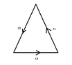
$$\iint_{\Omega}\left [u_{tt}(x, t)-c^2u_{xx}(x, t)\right ]dxdt=\int_{\partial{\Omega}}\left [-u_t(x, t)dx-c^2u_x(x, t)dt\right ]=\int_{C_1} [ \ \ ]+\int_{C_2} [ \ \ ]+\int_{C_3} [ \ \ ]$$

$(\int_{C_1} [ \ \ ]=cu(x_0, t_0), \int_{C_2} [ \ \ ]=cu(x_0, t_0), \int_{C_3} [ \ \ ]=0)$

View attachment 4135

$$\int_{C_3}[-u_t(x, 0)dx-c^2u_x(x, 0)dt], \text{ where } u_t(x, 0)=0, u_x(x, 0)=0$$ $$C_1: x+ct=x_0+ct_0 \Rightarrow dx+cdt=0$$
$$\int_{C_1}(-u_tdx-c^2u_xdt=\int_{C_1}-u_t(-cdt)-c^2u_x\left (-\frac{dx}{c}\right )=\int_{C_1}cu_tdt+cu_xdx=c \int_{C_1}u_tdt+u_xdx=c\int_{C_1}du=c(u(x_0, t_0)-u(x_0+ct_0, 0))\overset{ u(x_0+ct_0, 0)=0 }{ = }cu(x_0, t_0) \tag 2$$ $$2cu(x_0, t_0)=\int_0^{t_0}\int_{x_0-ct_0+ct}^{x_0+ct_0-ct}f(x, t)dx$$

$$u(x_0, t_0)=\frac{1}{2c}\iint_{c(x_0, t_0)}f(x, t)dxdt$$

I got stuck at the following:

Could you explain to me the first graph?? (Wondering)

Why are the limits of the integral at the relation $(1)$ the following: $x_0-ct_0+ct$ and $x_0+ct_0-ct$ ?? (Wondering)

Why does it stand at the relation $(2)$ that $u(x_0+ct_0, 0)=0$ ?? (Wondering)
 

Attachments

  • GreenT.png
    GreenT.png
    4.6 KB · Views: 55
  • c.png
    c.png
    2 KB · Views: 57
Physics news on Phys.org
  • #2
mathmari said:
Could you explain to me the first graph?? (Wondering)

Hey mathmari! (Mmm)

The first graph shows how the area $\Omega$ is chosen, which is a triangle.

Since we're talking about the wave equation, it makes sense to have 1 point at $(x_0,t_0)$ where a wave would start.
And to let it expand in both directions with speed $c$ for 2 more points at time $t$.
In the negative direction the wave will travel to $x_0 - c(t - t_0)$, while in the positive direction it will travel to $x_0 + c(t - t_0)$. (Thinking)
Why are the limits of the integral at the relation $(1)$ the following: $x_0-ct_0+ct$ and $x_0+ct_0-ct$ ?? (Wondering)

It's how we set up a line integral.
The left side the triangle is given by $x = x_0 - c(t - t_0)$ with $t_0 \le t \le t_1$ for some unspecified $t_1$. (Nerd)
Why does it stand at the relation $(2)$ that $u(x_0+ct_0, 0)=0$ ?? (Wondering)

Because the boundary condition $u(x, 0)=0$ is given for any $x \in \mathbb R$.
That is, at time $t=0$ there is no wave yet. (Wasntme)
 
  • #3
I like Serena said:
The first graph shows how the area $\Omega$ is chosen, which is a triangle.

Since we're talking about the wave equation, it makes sense to have 1 point at $(x_0,t_0)$ where a wave would start.
And to let it expand in both directions with speed $c$ for 2 more points at time $t$.
In the negative direction the wave will travel to $x_0 - c(t - t_0)$, while in the positive direction it will travel to $x_0 + c(t - t_0)$. (Thinking)
When we don't have the wave equation as for example at the following problem:
$$u_{tt}(x, t)-u_{xt}(x, t)=f(x, t), x \in \mathbb{R}, t>0 \\ u(x, 0)=0, x \in \mathbb{R} \\ u_t(x, 0)=0, x \in \mathbb{R}$$
do we take the points $x_0 - (t - t_0)$ and $x_0 + (t - t_0)$ ?? (Wondering)

I like Serena said:
Because the boundary condition $u(x, 0)=0$ is given for any $x \in \mathbb R$.
That is, at time $t=0$ there is no wave yet. (Wasntme)

Oh yes, you're right! (Blush)
 
  • #4
For the problem $$u_{tt}(x, t)-u_{xt}(x, t)=f(x, t), x \in \mathbb{R}, t>0 \\ u(x, 0)=0, x \in \mathbb{R} \\ u_t(x, 0)=0, x \in \mathbb{R}$$ do we have the following?? The two characteristics are $x=x_0$ and $x+t=x_0+t_0$.

The region $\Omega$ is the triangle:

View attachment 4138

$$\iint_{\Omega}[u_{tt}(x, t)-u_{xt}(x, t)]dxdt=\iint_{\Omega}f(x, t)dxdt=\int_0^{t_0} \left (\int_{x_0}^{x_0+t_0-t}f(x, t)dx\right )dt$$

$$\iint_{\Omega}\left [\frac{\partial{Q}}{\partial{x}}-\frac{\partial{P}}{\partial{t}}\right ]dxdt=\int_{\partial{\Omega}}Pdx+Qdt$$

$$Q(x, t)=-u_t \\ P(x, t)=-u_t$$

$$\iint_{\Omega}\left [u_{tt}(x, t)-u_{xt}(x, t)\right ]dxdt=\int_{\partial{\Omega}}\left [-u_t(x, t)dx-u_t(x, t)dt\right ]=\int_{C_1} [ \ \ ]+\int_{C_2} [ \ \ ]+\int_{C_3} [ \ \ ]$$

View attachment 4139

$$C_1: x+t=x_0+t_0 \Rightarrow dx+dt=0 \Rightarrow dx=-dt$$
$$\int_{C_1} \left [-u_t(x, t)dx-u_t(x, t)dt\right ]=\int_{C_1} \left [u_t(x, t)dt-u_t(x, t)dt\right ]=0$$

$$C_2: x=x_0 \Rightarrow dx=0$$
$$\int_{C_2} \left [-u_t(x, t)dx-u_t(x, t)dt\right ]= \int_{C_2} \left [-u_t(x, t)dt\right ]=-\int_{C_2} \left [du\right ]=u(x_0, t_0)-u(x_0, 0)=u(x_0, t_0)$$

$$C_3: t=0 \Rightarrow dt=0$$
$$\int_{C_3} \left [-u_t(x, 0)dx-u_t(x, 0)dt\right ]=0$$

So, we have $$u(x_0, t_0)=\int_0^{t_0} \left (\int_{x_0}^{x_0+t_0-t}f(x, t)dx\right )dt$$

Is this correct?? (Wondering) Could I improve something?? (Wondering)
 

Attachments

  • infreg.png
    infreg.png
    2.8 KB · Views: 48
  • region.png
    region.png
    1.9 KB · Views: 44
Last edited by a moderator:

Related to Differential equation - Green's Theorem

1. What is a differential equation?

A differential equation is a mathematical equation that relates an unknown function to its derivatives. It describes the relationship between a function and its rate of change.

2. What is Green's Theorem?

Green's Theorem is a fundamental theorem in multivariable calculus that relates the line integral of a two-dimensional vector field around a simple closed curve to a double integral over the region enclosed by the curve. It allows for the evaluation of certain line integrals by converting them into simpler double integrals.

3. How is Green's Theorem used in differential equations?

Green's Theorem can be used to solve certain types of differential equations, such as those involving a two-dimensional vector field. It allows for the transformation of a line integral into a simpler double integral, making it easier to solve.

4. What are the applications of Green's Theorem?

Green's Theorem has a wide range of applications in physics, engineering, and other fields. It is commonly used in fluid dynamics, electromagnetism, and to solve problems involving the calculation of work or energy.

5. Is Green's Theorem applicable to all types of differential equations?

No, Green's Theorem is only applicable to certain types of differential equations, specifically those involving a two-dimensional vector field. It cannot be used to solve all differential equations, but it is a useful tool in many applications.

Similar threads

Replies
1
Views
1K
  • Differential Equations
Replies
7
Views
453
  • Differential Equations
Replies
1
Views
835
  • Differential Equations
Replies
1
Views
811
  • Differential Equations
Replies
6
Views
1K
  • Differential Equations
Replies
1
Views
721
Replies
1
Views
1K
Replies
1
Views
1K
  • Calculus and Beyond Homework Help
Replies
4
Views
630
Replies
8
Views
1K
Back
Top